2.4.3 Defining Arbitrary Curves
Arbitrary curves are curves defined by a vector expression of voltages and/or currents or from an expression of existing graph waveforms. The input vectors to the expression can come from a number of sources, including interactive selection of schematic nodes or waveforms. As the easiest way to generate these curves is with a fixed schematic probe, this method is be presented first.
To download the examples for Module 2, click Module_2_Examples.zip
In this topic:
What You Will Learn
- How to use fixed schematic probes to plot arbitrary expressions.
- You can plot the power in any device with the menu item.
- How to generate curves which are expressions of existing graph curves.
- How to generate curves which are arbitrary expressions containing multiple vectors selected from the schematic.
Getting Started
Creating Arbitrary Curves From Fixed Schematic Probes
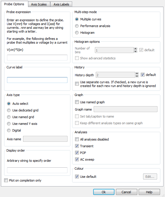
The Arbitrary Probe is a very powerful fixed schematic probe with an automatically created symbol. To use this probe, you enter a expression of voltages and currents in the dialog box, and the program creates a symbol which has a pin for each voltage, and a pair of pins connected by a 0-volt DC source for each current. Voltages are entered in the expression as V(nnn), and currents as I(nnn), where nnn is a unique string identifier. After entering the expression and closing the dialog box, the program creates a symbol with the correct pins and with the graphing statements which implement the arbitrary expression.
Exercise #1: Create and Place Arbitrary Probe
- Open the 2.4_SelfOscillatingConverter_POP_Tran.sxsch schematic.
- From the schematic menu, select .Result: The arbitrary probe dialog opens.
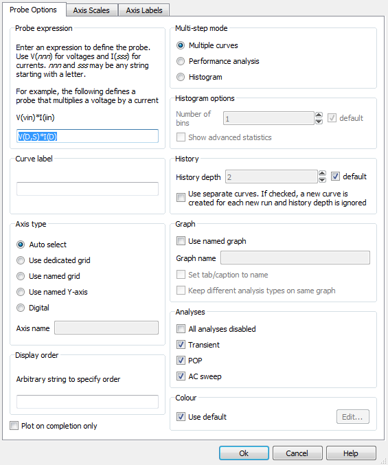
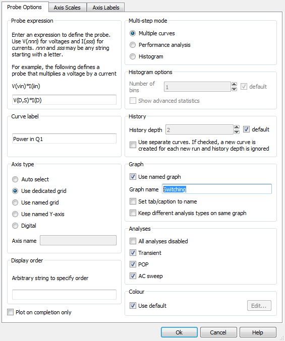
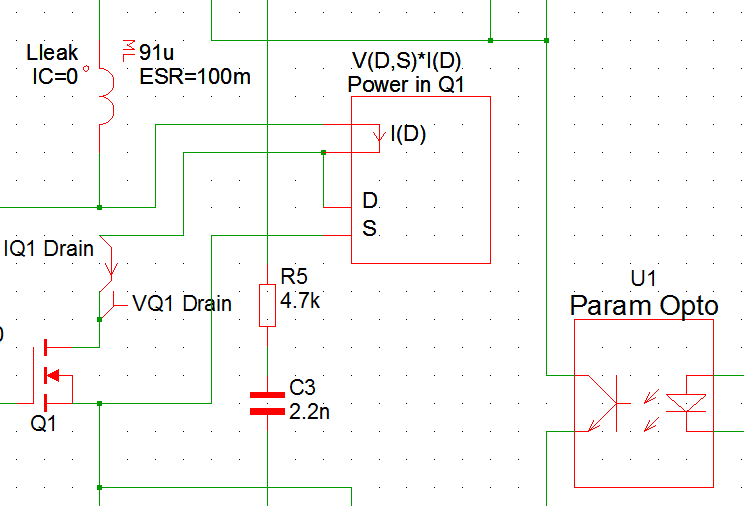
- In the Probe expression box, enter the expression: V(D,S)*I(D).
This is a shorter expression than the full expression: \[ \text{P} = \left(
V_{DRAIN} - V_{SOURCE} \right) \times I_{DRAIN} \] The syntax: V(D,S) is
equivalent to V(D)-V(S). You will see that this shorter expression
creates a smaller probe symbol than you would see with the full expression. In
this case, the smaller probe is easier to place and wire on the schematic. The
configured dialog should appear as:
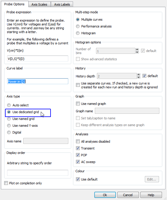
- In the Curve label box, enter Power in Q1.
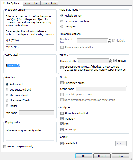
- In the Axis type box, select the Use dedicated grid radio
button.
- To the right of the Axis type box is the Graph box. In the Graph
box, select Use named graph and in the Graph name box, enter
Switching. The configured dialog now appears as:
- Click Ok.Result: The program parses the Probe expression, and creates a schematic probe which has the correct pins and enters into a place mode:
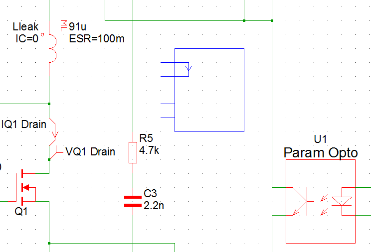
- Place the probe in the approximate location shown above. Next, you will wire the probe into the existing schematic components.
- Wire the arbitrary probe to the schematic:
- First, select the 1-grid square length wire which connects the IQ1 Drain
probe to the transformer network. To accomplish this, you will need to
press and hold the Shift key while dragging a box around the wire.
This tells the program to only select wires, not the default which is
wires and symbols.
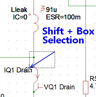 Result: Just one grid square of wire is selected.
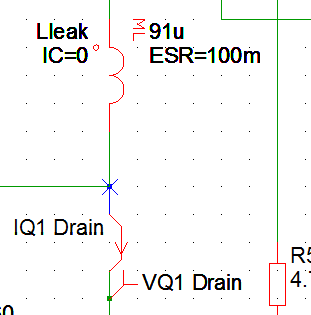
- Press the Delete key to delete this wire.
- Now wire the probe into the existing circuit. The final wiring should
appear equivilent to:
- First, select the 1-grid square length wire which connects the IQ1 Drain
probe to the transformer network. To accomplish this, you will need to
press and hold the Shift key while dragging a box around the wire.
This tells the program to only select wires, not the default which is
wires and symbols.
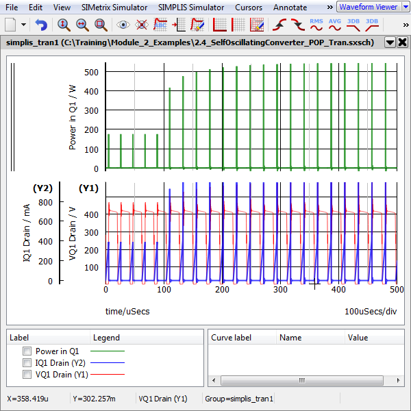
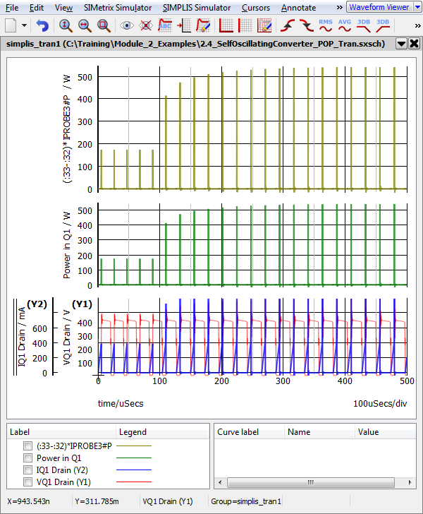
- Press F9 to run the simulation.Result: The power expression is plotted as a green curve above the drain voltage and drain current waveforms.
Creating Arbitrary Curves Interactively
In the first exercise, you created an arbitrary probe symbol, wired it to the schematic and ran a simulation, producing a curve which approximates the power dissipated in the MOSFET. In this case we knew the expression we wanted to plot, and this is not always the case. There are occasions where you will want to generate curve interactively after the simulation completes. In the next example, you will generate the same arbitrary curve using the Define Curve Dialog.
Using the Define Curve Dialog, you can enter expressions defining the Y and X axis of the curve. By default the dialog assumes that the X axis is time (or frequency) and that the user must enter the expression for the Y axis. You can enable the X-Y plot by selecting the X-Y Plot check box. The expressions can contain vector names and a set of built-in functions. The results of the X and Y expressions are expected to be vectors and are plotted on the graph and axis you specify in the dialog.
Exercise #2: Using The Define Curve Dialog to Plot the Power in a Device
- This exercise starts with the schematic 2.4_SelfOscillatingConverter_POP_Tran.sxsch opened, and with the simulation data from the last step of the first exercise.
- From the menu bar, select . Result: The Define Curve Dialog opens:
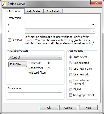 Note: The Define Curve dialog is interactive, that is, you can click on the waveform viewer or the schematic to automatically populate the dialog X and Y fields with vectors. This is different than other dialogs which steal focus and therefore prevent you from interacting with the other SIMetrix/SIMPLIS windows while the dialog is open.
 - Click in the Y field at to top of the dialog and press ( to start the expression.
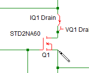
- On the schematic, left-click on the drain connection of the MOSFET Q1:
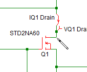 Result: The dialog is populated with the drain voltage node, :33.Note: Your node numbers might be different, depending on how you re-wired the arbitrary probe in the first exercise.
 - Next, type a minus character, - so that the Y expression is (:33-.
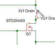
- On the schematic, left-click on the source connection of the MOSFET Q1:
 Result: The dialog is populated with the source voltage node, :32.
 - Type )*, making the Y expression (:33-:32)*
- Press and hold the shift key while left-clicking on the positive side of the
IQ1 Drain current probe:
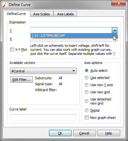
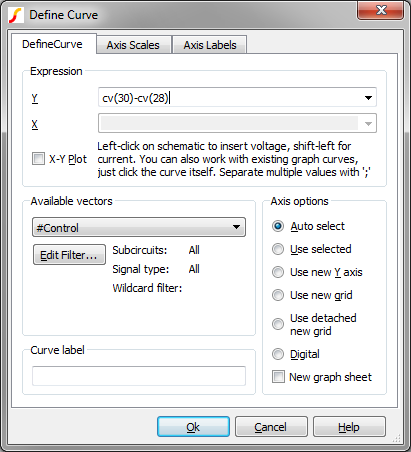
 Result: The dialog is populated with the probe current, IPROBE3#P, the final Y expression is (:33-:32)*IPROBE3#P. The dialog should now appear as shown below:
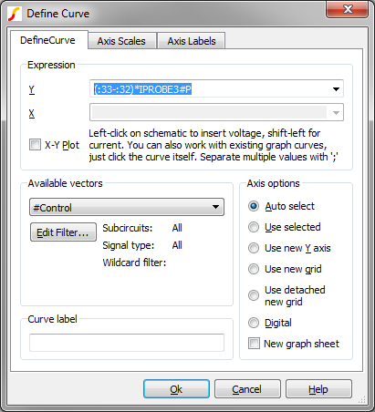
- To put the curve on a new grid above the existing grid before you accept the
dialog and plot the curve, select the Use new grid radio button as shown
below:
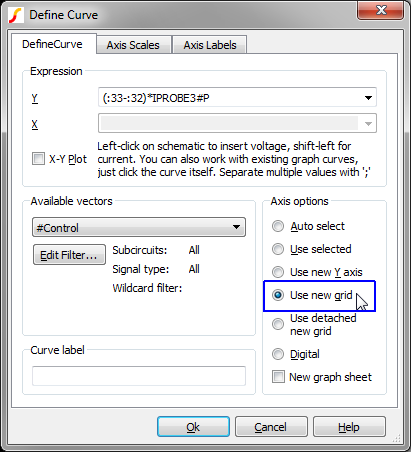
- Click Ok. Result: The power in Q1 is plotted on a new grid above the arbitrary probe you created in the first exercise. Because you didn't specify a curve name, the program labeled the curve with the expression which created it.
The above procedure used the bare minimum of steps. At any point in the process, you can hand type into the expression box. The Define Curve Dialog allows you to specify much more than just the curve expression, as you will see with the next example.
Exercise #3: Expression History and Curve Annotation
One useful feature of the Define Curve Dialog is that the system remembers the previously plotted expressions. In this example, you will delete the curve you just created and add it with a more useful name than the actual vector expression, which is (:33-:32)*IPROBE3#P.
- Select the curve you just created with the curve label (:33-:32)*IPROBE3#P. You can select curves by clicking on the curve in the waveform viewer.
- Press the Delete key. Result: The curve and axis are deleted.
- From the waveform viewer menu bar, select
Result: The Define Curve Dialog opens.
- Select the Y expression combo box pull down as shown below:
Notice that the curve expression you defined in the first example is remembered and is available to be plotted.
- Select the previously used curve expression.
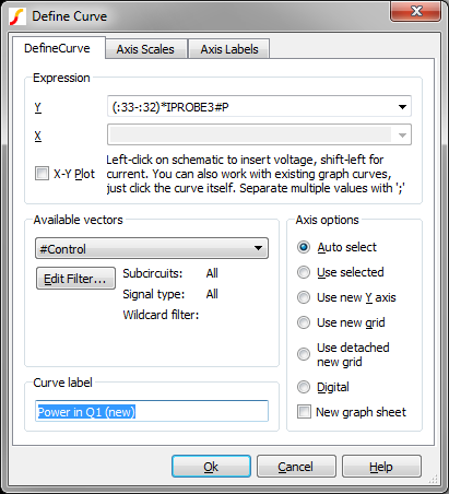
- In the Curve label field, type an appropriate curve label, such as Power in Q1
(new). The resulting dialog is shown below:
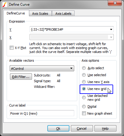
- , To put the curve on a new grid above the existing grid as you did with the
first example, select the Axis/Graph Options tab and select the Use new
grid radio button as shown below:
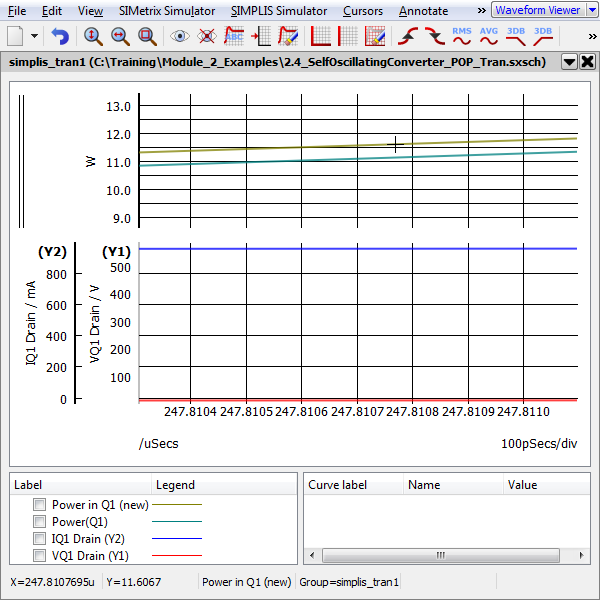
- Click Ok. Result: The Power in Q1 (new) curve is added to a new grid on the waveform viewer. While the vector information is identical to the previous curve, the curve label is much shorter and its intuitive that the curve represents the power dissipated in Q1.
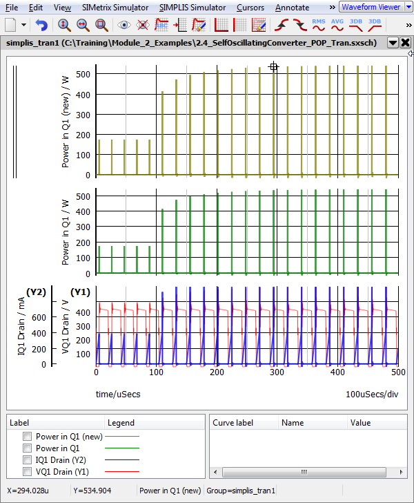
In the first three exercises, you plotted the power in Q1 taking into account only the power from the drain current and drain-to-source voltage product. SIMetrix/SIMPLIS has a very powerful probe feature which automatically plots the power in a device, taking into account all pin currents and voltages. In the next exercise, you will compare the power dissipation generated using this method vs. the Define Curve method.
Exercise #4: Compare with the Power In Device Function
The schematic menu automatically generates the power in a single device. This includes any device implemented as a subcircuit, such as a hierarchical schematic component. To probe the power in the MOSFET Q1,
- With the graph open from the last example, select from the schematic menu.
- Move the mouse over to the MOSFET Q1:
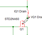
- Left-click the mouse. Result: A curve with label Power(Q1) is added to the waveform viewer. This curve is added to the selected grid, which is the upper grid on the waveform viewer.
Exercise #5: Difference of Two Graph Curves
At this point the waveform viewer has the drain voltage and draing current curves, and the three curves you added, one created with the Arbitrary Fixed Schematic Probe, one created with the Define Curve Dialog, and one created with the Power In Device random probe. Because of the large magnitudes of these curves, comparing the difference between them is quite difficult. In this example, you will plot the difference of the two power curves.
- Select the power curve in the middle grid.
- Press delete to remove this curve and it's grid.
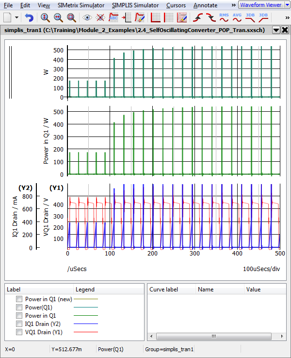
- Zoom in on the power curves in the upper grid using the box select:
- Press and hold the left mouse button while dragging the mouse to create a
box selection.
- Repeat until the two curves separate on the waveform viewer: Result: Your curves will appear differently than the image below depending on which portion of the curve you zoomed in on.
- Press and hold the left mouse button while dragging the mouse to create a
box selection.
- Once you can distinctly see the two curves, you can add the difference curve. From the menu bar, select
- In the waveform viewer, left-click on the curve with the label Power(Q1)
Result: The Y expression is updated with cv(n), where n is an integer. The integer value is not important.
- Type a minus character (-) so that the expression is now cv(n)-.
- In the waveform viewer, left click on the curve with the label Power in Q1
(new)
Result: The Y expression is updated with cv(m), where m is an integer. The dialog should be configured as below:
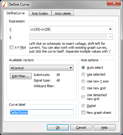
- Add a descriptive curve label, such as Delta Power
- As with the first two exercises, you should put the curve on a new grid above the
existing grid. Select the Axis/Graph Options tab and select the Use new
grid radio button as shown below:
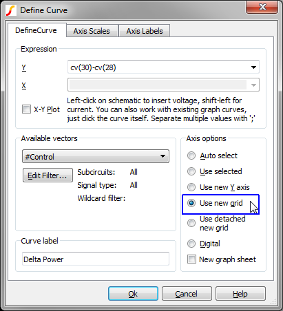
- Click Ok. Result: A new curve is added to a new grid above the existing grids. This curve represents the difference in power dissipation between the two methods, and is calculated from the two existing power curves, which were themselves calculated from the raw voltage and current vectors.
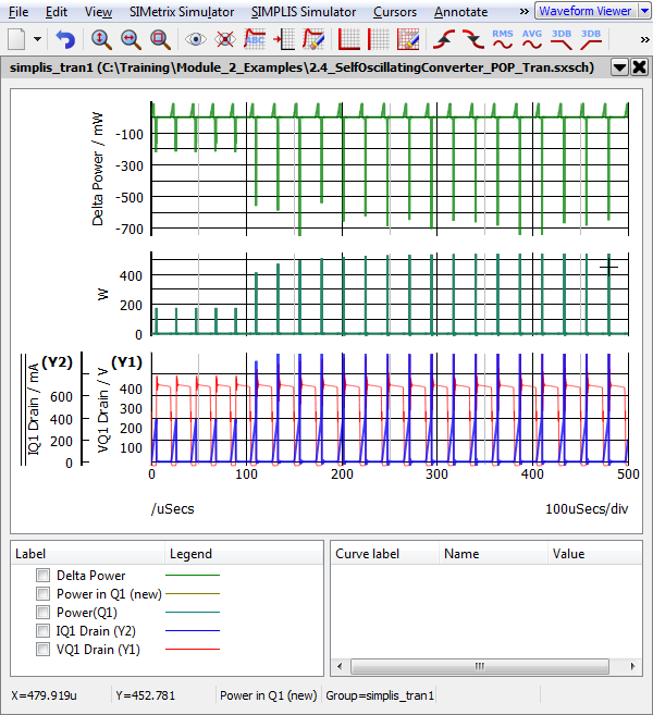
- You can press the Home key to zoom to the full extent of the waveform viewer.
You can now zoom on the waveform viewer and easily see that the power difference is the power coming into and out of the gate terminal.
Conclusions and Key Points to Remember
- The arbitrary fixed probe allows you to automatically plot an expression of voltages and currents after each simulation run.
- The Define Curve dialog allows you to interactively plot mathematical expressions of different vectors.
- When creating curves interactively, the curve to be plotted can be made up of existing graph curves, schematic nodes, or a combination of both.