2.3 Design an Inductor Using MDM
In this section of the tutorial you create an initial inductor design for the Buck converter. Then you will perform post-processing in MDM after simulating the schematic to obtain a detailed inductor loss estimate.
In this topic:
Key Concepts
This topic addresses the following key concepts:
- The Level 2 model only adds a DC winding resistance (ESR) to the inductor symbol inside the schematic. In order to obtain more accurate winding and core losses, post-processing must be performed in MDM.
- MDM post-processing occurs after the circuit simulation in SIMPLIS, and must be set up properly to take in a portion of the resulting circuit simulation waveforms.
- MDM provides a calculation of the average power loss in the inductor over the simulation period provided. Therefore, for meaningful results, you must make sure that you are providing MDM with steady-state converter waveforms over an integer number of steady-state cycles (preferably one).
What You Will Learn
In this topic, you will learn the following:
- How to design an inductor using SIMPLIS MDM that meets your design requirements.
- How to properly set-up and perform post-processing in MDM to obtain detailed inductor loss estimates.
- How to analyze the results MDM provides.
2.3.1 Design the Inductor
Remember, you want an inductor with an inductance in between 600 and 700 nH. To create an initial inductor design for the Buck converter, follow these steps:
- Double-click the symbol L1.
- In the resulting dialog, switch the model to Level 2.
-
Check the Write MDM generated model parameters to all lower model levels? checkbox.
- Click the Create with SIMPLIS MDM... button.
- In the MDM main window, go to the Core tab, if it is not already showing.
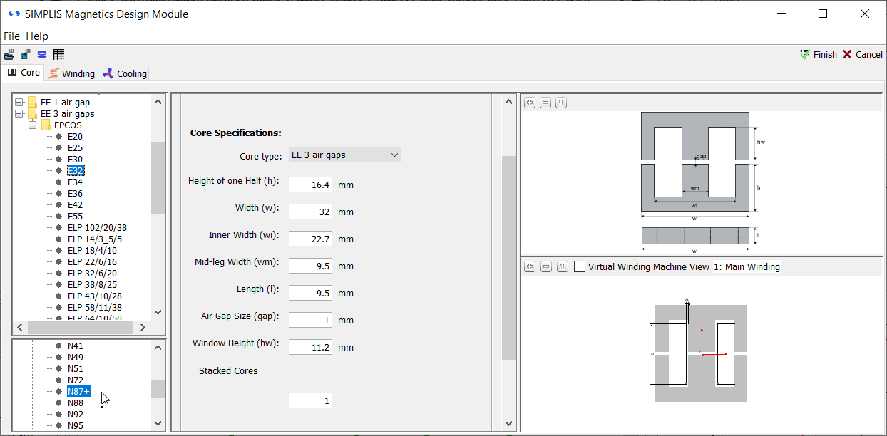
- In the core geometry selection menu tree, select EE 3 air gaps > EPCOS > E32. You have selected the E32 core with three variable air gaps for this design.
- In the core material selection menu tree, select Ferrite > EPCOS > N87+. The E32 core is commercially available made from the N87 material.
- In the lower right panel, click
 to re-center the inductor visualization.
 - In the middle panel showing the core dimensions, scroll down until you see the
input field for Air Gap Size (gap): and set it to 1. Result: The core tab should now look like this:
- Open the MDM Status Window. Move it to the side so you can see both it and the entire MDM main window.
- Switch to the Winding tab.
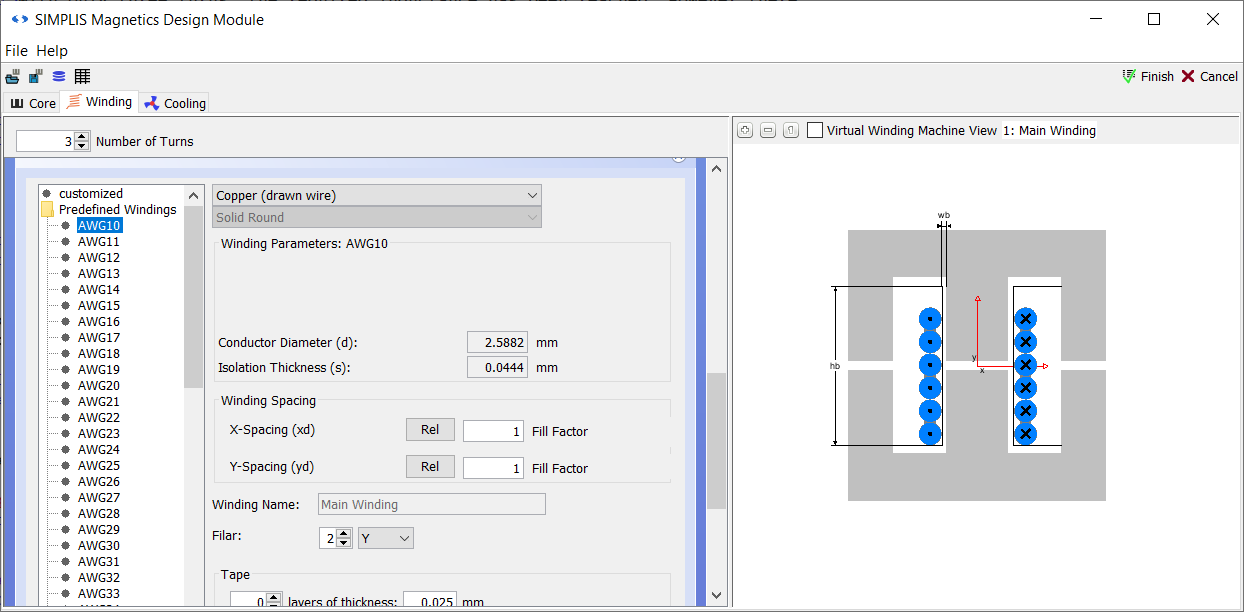
- Scroll down in the left panel until you see the third unnamed sub-panel. In the wire selection tree menu, select Predefined Windings > AWG10.
- Increase the number of turns to 3. Result: In the status window, an inductance of 878 nH for this inductor is displayed.
- Since the inductance is too large with just three turns, try a smaller core. Go back to the Core tab.
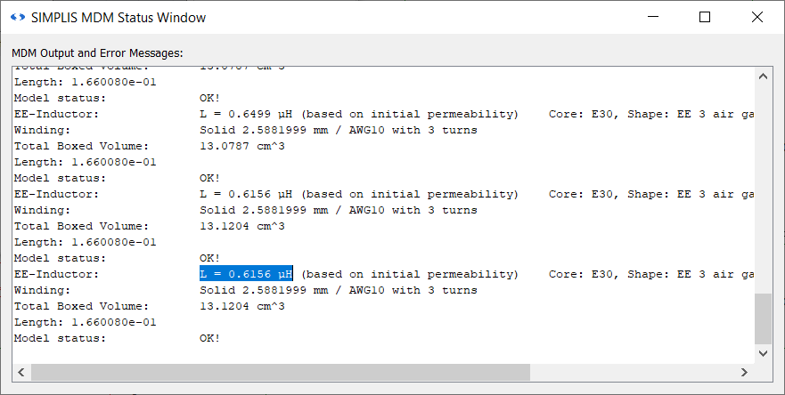
- Select a smaller core: EE 3 air gaps > EPCOS > E30.
- Increase the air gap of the core to 1.1 and press Enter. Result: In the status window, an inductance of 615.6 nH for this inductor is now displayed:
- You now have an acceptable initial inductance. Go back to the Winding tab.
- With only three turns, the required inductance has been reached. However there is still a lot of free space in the core's winding window. More copper can therefore be added, but there is no need for extra turns. To add more copper without adding turns, you can make the winding multi-filar. MDM allows you to create a bifilar, trifilar, ..., n-filar winding. On the panel next to the wire selection menu tree, find the spinner named Filar:.
- From the drop-down box next to this spinner, select Y.
- Increase the Filar spinner to 2. Result: The winding tab should now look like this:
- Close the MDM Status Window.
- In the upper right corner of the main MDM window, click Finish.
You have now saved an MDM physical model of the inductor to the symbol L1. From this physical model, a Level 2 model for L1 has been extracted. To see this, double-click on L1. You should see the following:
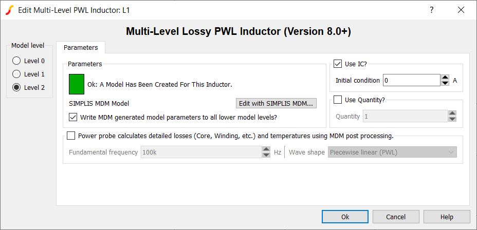
You can see that the model status box is green and that model status is Ok: A Model Has Been Created For This Inductor.
Make sure that the checkbox Power probe calculates detailed losses is unchecked. Then click OK to close the dialog.
2.3.2 Add a Power Probe
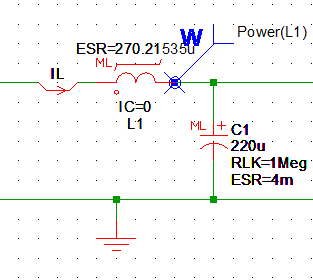
You can see now that the ESR of the Level 2 model generated by MDM is displayed on the schematic above L1. In order to measure losses, you must add a power probe, as is standard procedure in SIMPLIS when you want to measure the power loss in a component. To do so,
- In the Part Selector, double-click on Probes > Power Probe.
- Put the power probe on the right pin of L1:
- Double click the probe you just placed.
- Make sure that in the Edit Probe dialog that appears, under
Analyses the boxes Transient and POP are checked:
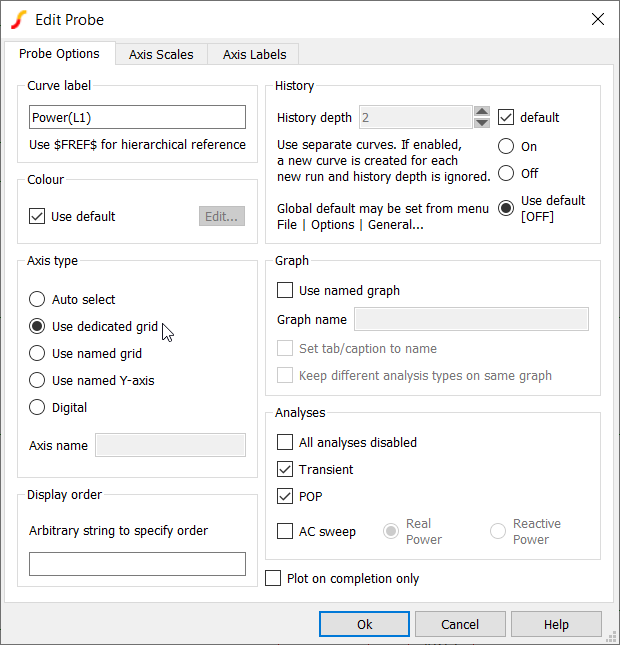
- This will ensure that the power loss of the inductor is displayed in the Waveform Viewer when the simulation is run. Now under Axis type select Use dedicated grid. Click OK.
2.3.3 Add Mean Measurement to Power Probe
Next you will add the mean measurement to the power probe. This measurement will be performed after every simulation, with the mean value for the power dissipation output to the waveform viewer.
To add the mean measurement to the Power(L1) probe, follow these steps:
- Select the power probe Power(L1).
- Right click and run the menu Edit/Add Measurement....
- Select the Mean measurement in the drop down list.
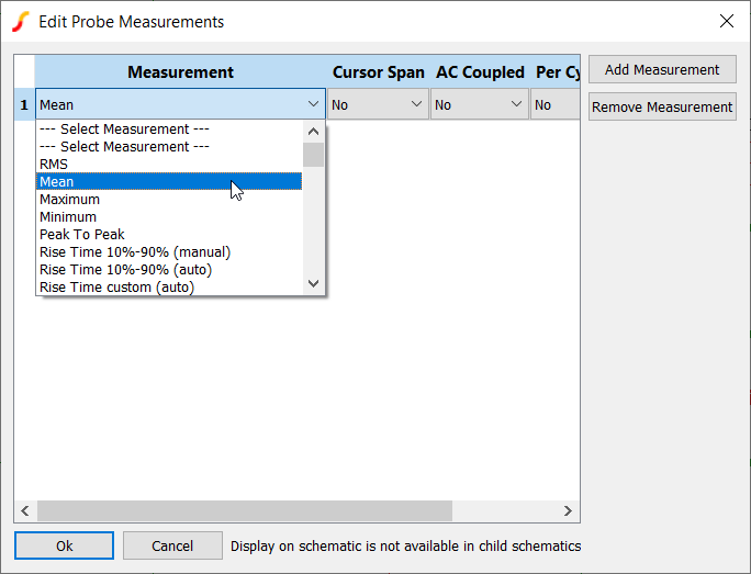
- Click Ok.
2.3.3 Run the Simulation Without MDM Post-Processing
Now you will run the simulation using the power probe to calculate inductor losses based on the Level 2 model, but without using MDM for post-processing. This was previously the only way to calculate losses in SIMPLIS. In the previous section you added a mean value measurement to the power probe. In this section you will see that this measurement only measures the loss due to the RMS current in the inductor.
- Press F9 to run the simulation.
Result: The results appear in the Waveform Viewer, including now the power loss of the inductor.
- Click on the Waveform Viewer.
Result: The menu bar will change to reveal the Measure menu.
- In the measurement pane in the lower right corner of the Waveform Viewer, scroll until you find the measurement for Power(L1) Mean:
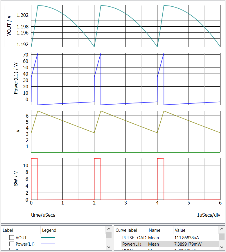
You will see that the power probe has measured an average loss in the inductor of 7.39mW.
However, it is very important to note that the ESR of the Level 2 model that is shown on the schematic is based on the DC resistance of the inductor winding ONLY. Therefore, the loss measurement which you just performed does NOT include core losses, AC winding losses, and losses due to proximity effect.
In order to obtain those detailed losses, you must run MDM post-processing after the circuit simulation.
2.3.4 Run the Simulation With MDM Post-Processing
Now you will run set up and run MDM post-processing after the circuit simulation to obtain a detailed calculation of inductor losses - including core losses, AC winding losses, and proximity effects, as well as the inductor temperature, none of which you can obtain by just using a regular SIMPLIS power probe as in the previous sub-section.
In post-processing, MDM calculates average inductor loss over a specified section of the circuit simulation waveform. An instantaneous power loss waveform, as given by the regular power probe, is not provided. Therefore, for the results to be meaningful, you want to make sure that MDM uses an integer multiple of the converter's steady-state cycle for the calculation. The more cycles are included, the longer the calculation will take, so the ideal number of cycles is one. Calculating average power loss over one steady-state cycle will give you the average power loss in the inductor when the converter is in steady-state.
Note that MDM assumes that you have set-up the post-processing to produce meaningful results. It will calculate the power over a quarter- or half-cycle, over 3.37 cycles or during converter startup if you so instruct it to. While average power loss in steady-state is what you are usually most interested in, if you run post-processing on a different type of waveform, it's up to you to make sense of the results properly.
For the inductor, MDM needs both the current and voltage waveform of the inductor. You do not need to necessarily plot these explicitly to the Waveform Viewer in SIMPLIS. In this example, you will notice that while the inductor current is plotted, the inductor voltage is not. MDM will automatically acquire the waveforms it needs regardless of what you plot to the Waveform Viewer.
To set up MDM post-processing for the inductor in the Buck converter,
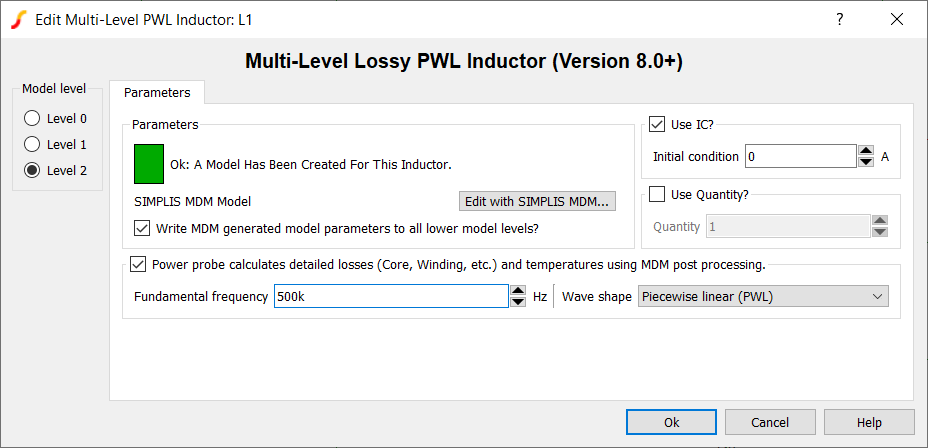
- Double-click L1
Result: The Edit Multi-Level PWL Inductor dialog opens, showing the Level 2 model.
- Check the Power probe calculates detailed losses (Core, Winding, etc.) and temperature using MDM post processing checkbox.
Result: The two fields below the checkbox are now enabled.
- The Fundamental frequency field determines how much of the circuit simulation waveform is sent for post-processing in MDM. MDM will take the last fundamental period (calculated as the inverse of the entered fundamental frequency) of the simulation waveforms to use for the post-processing calculations. As noted earlier, it is best if this is a single steady-state converter cycle. In a Buck converter, a steady-state cycle is a switching cycle. Since the switching frequency of this converter is 500kHz, for Fundamental frequency enter 500k.
- MDM must also be aware of the shape of the waveform. This is needed for the accurate calculation of core losses. You must specify this in the Wave shape drop-down menu.
Since a rectangular voltage is applied to an inductor in a buck converter causing it to conduct a triangular current, set the Wave shape to Piecewise linear (PWL).
The dialog should then look like this:
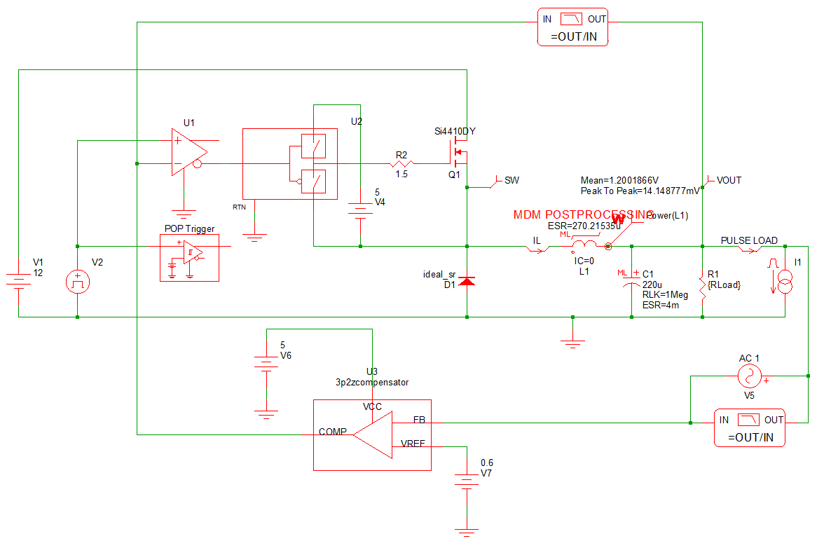
- Click OK. Result: The label MDM POSTPROCESSING appears above L1:
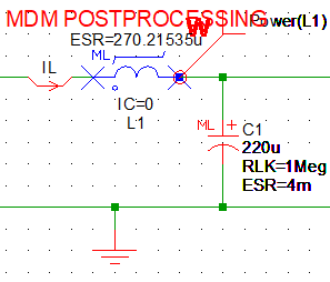
- Press F9 to run the simulation.
Result: After the circuit simulation completes, a window indicating that MDM post-processing appears, displaying "Calculating losses for L1...".
- Once MDM post-processing is finished, the MDM Results window will appear:
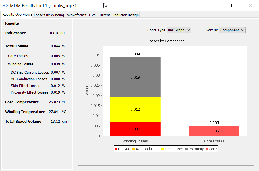
By default, the MDM Results window is open to the Results Overview tab. To the left, it shows the initial inductance, a textual breakdown of the different types of losses in the inductor, and also the core and winding temperatures, as well as the boxed volume of the inductor. Note that the DC Bias Current Losses are given as 0.007W - the same as you previously measured with the power probe. However the actual total losses are much higher - 0.044W. You can see that MDM post-processing can give you a much better insight into what the inductor losses will be than you can obtain by just setting an ESR in the schematic.
You might ask yourself if you could not obtain the same results by just setting the ESR of L1, in a Level 1 model, to the required value to obtain a loss of 44mW. While this is of course possible, there are two limitations with this approach. First, this would not provide a detailed loss analysis which you can use to improve your inductor design. Second, you do not know this value of ESR ahead of time. While it is easy to calculate the DC winding resistance once a physical model of the inductor is created in MDM, the AC winding losses and the core losses depend on many factors that are operating-point dependent: frequency, flux density inside the core, temperature, the duty ratio of the waveforms, and DC current. Thus the "ESR" for each operating point would be different. MDM post-processing will give you accurate loss estimates for different operating points without the need to adjust the ESR of the inductor in the schematic.
There are some other important things to note:
- The MDM Results window does not block SIMetrix/SIMPLIS like the main MDM window does. You can close it at any time, or just minimize it or leave it in the background. In the MDM Beta version, you cannot bring back a Results window you have closed. Once you close it, the only way to regenerate it is to re-run the simulation.
- Checking the post-processing checkbox in the Edit Multi-Level PWL Inductor dialog converts an "ordinary" power probe into an "MDM post-processing" power probe. Note that it not sufficient for just the box to be checked to perform MDM post-processing: both a power probe must be placed on the symbol and the checkbox must be checked.
- With the MDM POSTPROCESSING label above the inductor symbol, you can easily see by looking at a schematic for which symbols MDM post-processing is selected, and by extension, which symbols have a valid MDM Level 2 model defined.
- In the title bar of the MDM Results window you can see which symbol the results are for and to which SIMPLIS simulation group they refer. In this example the title is MDM Results for L1 (simplis_pop3). Therefore when you have several windows open, you can refer to this to figure out for which symbol and which simulation run the results are.
2.3.5 Analyze the MDM Results
Now you can analyze the MDM inductor results in more depth. You can see that the DC winding losses and core losses are quite low at about 7mW and 5mW, respectively. However the total winding losses are quite high, with proximity losses dominating at 19mW. To gain more insight into why proximity losses are so high, switch to the Losses By Winding tab of the MDM Results window:
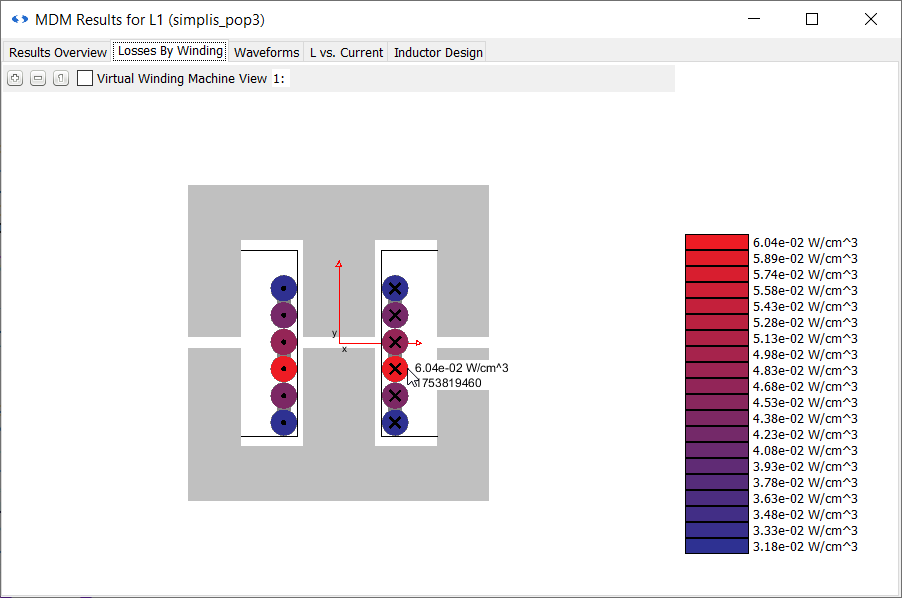
Here the loss density of each turn (in W/cm3) of the winding is displayed. The more red the turn, the higher the losses inside it. Note that the scale to the right is relative and differs for each inductor and operating point. The most intensely red turn is the one with the most losses relative to the others - it does not necessarily mean that it's very hot.
You can see that the turns closest to the air gap have the highest loss density. This is the result of fringing flux field produced by the air gaps of the core. As the magnetic flux in the core travels across the air gap, it fringes and a field is generated inside the winding window which creates proximity losses in the winding. So despite using a large bifilar wire to reduce the winding resistance, the way the turns are arranged relative to the air gap produces significant winding losses.
Now switch to the Waveforms tab of the MDM Results window. Here the flux density inside the inductor core (in Tesla), the inductor current (in Amperes) and the inductor voltage (in Volts) are shown:
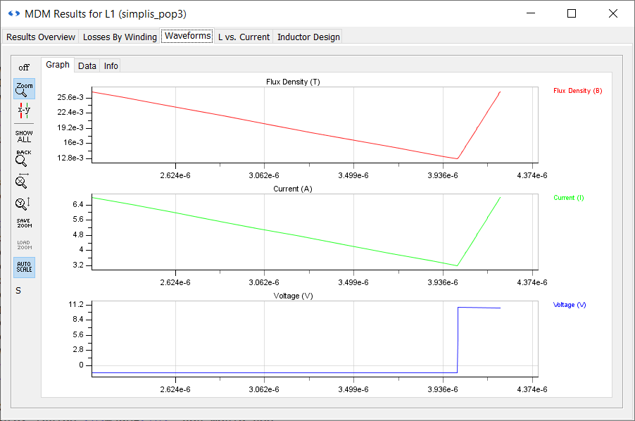
Note that the peak flux density is about 25mT. If you were to examine the N87+ material used for this inductor inside MagDB, you would see that the peak flux density of this material is given as 360mT. Also note that the peak current in the inductor is about 6.5A.
Now switch to the L vs. Current tab. Here the inductance of the inductor as a function of the current is shown:
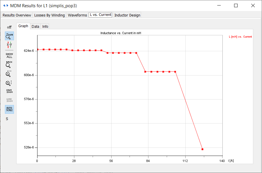
The inductance starts to drop off only after 48A, with another significant drop after 75A, and the inductor saturates only above 105A. This is many times higher than the peak inductor current in this converter. You can conclude from this, as well as from the peak flux density, that this inductor is using a core which is too large for this application. Indeed, if you go back to the Results Overview tab, you will see that the boxed volume is 13.12 cm3. A 7A, 600nH inductor can be much smaller. Additionally, you can see by looking at the core and winding temperatures that the inductor is quite cool, heating up less than 3 degrees above the ambient temperature of 25 degrees.
Therefore, there is a lot of room to improve this inductor design. You will do this in the next section: 2.4 Refine the Inductor Design Using MDM
Minimize or close the MDM Results window. Save the schematic as 2_my_buck_E30_core.sxsch.
A complete schematic with the inductor design developed in this section, set up for MDM post-processing, is available as 2.3_SIMPLIS_MDM_tutorial_buck_converter_E30core.sxsch in the zip archive of schematic files: