Synopsis of the Periodic Operating Point Analysis
As pointed out earlier, the periodic operating point analysis must be the first analysis specified in an input file. As a result, the initial capacitor voltages and initial inductor currents at the start of the periodic operating point analysis are the same as those specified in the device statements and any overriding initial conditions supplied in the .INIT statements. Then, the periodic operating point analysis tool carries out a sequence of time-domain transient simulation on the system. The actions of the periodic operating point analysis are summarized by the flow chart in Fig 10.3.
The transient analysis shown in Fig 10.3 is carried out indefinitely until the start of a new switching cycle is reached or until the value of the time variable has reached the parameter value of the maximum period set in the .POP statement. If the transient analysis fails to reach a condition to trigger the start of a new switching cycle before the maximum period is reached, an error message similar to the one shown below is either printed on the screen or to an error file. After the error message has been printed, SIMPLIS aborts its execution.
Periodic Operating-Pt Analysis:
Reaching a time duration equal to
'3.00000e-04' without registering the
triggering condition that defines
the start of a period. Check your
circuit and/or initial conditions.
If the transient analysis is able to reach a condition triggering the start of a new switching cycle, the next task to be performed is to determine whether the system has reached steady-state operation. This is accomplished by finding the difference between the values of each capacitor voltage and inductor current at the start and end of the finished transient analysis. If the differences are small enough to be negligible for all capacitors and inductors, the system is considered to be in steady-state operation and the periodic operating point analysis is considered successful and it is stopped.
If the system is not considered to be in steady-state operation, the periodic operating point analysis tool applies a proprietary algorithm to predict what the values of the capacitor voltages and inductor currents at the start of a switching cycle ought to be had steady-state operation condition been reached. After this prediction phase, another transient analysis is initiated and the whole algorithm is repeated until either steady-state condition has been reached or the maximum iteration limit as set in the POP_ITRMAX option has been reached. If the maximum iteration limit is reached, an error message similar to the following is either printed on the screen or to an error file and execution of SIMPLIS is halted.
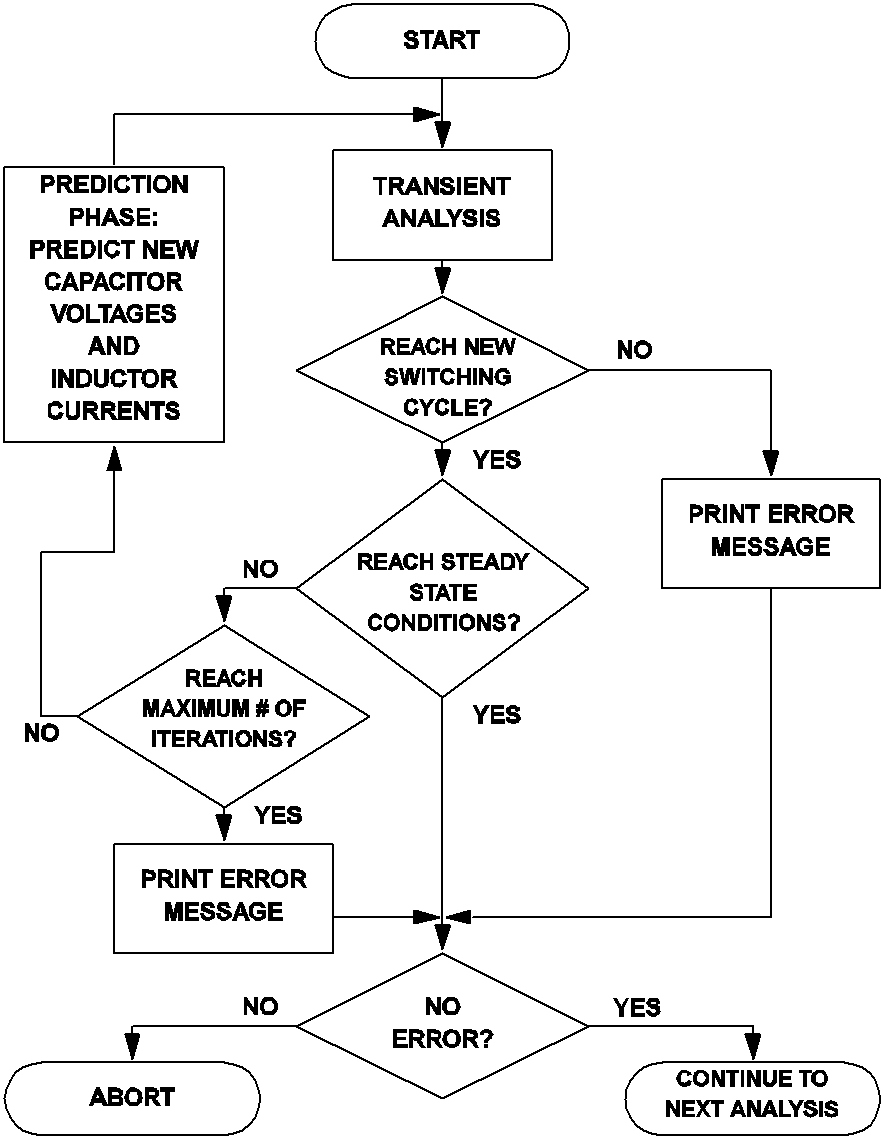 |
10.3 Actions carried out by the periodic operating point analysis tool |
Periodic Operating-Pt Analysis:
Unable to find a periodic operating
point after 20 attempts. Check your
input file for errors. A change in
the initial condition may be necessary.
During each iteration, or pass, of the algorithm shown in Fig 10.3, the periodic operating point analysis tool provides a glimpse of the progress of the analysis by printing out short messages on the screen. The messages on the screen from a typical successful periodic operating point analysis will be similar to the following:
PERIODIC OPERATING-POINT ANALYSIS
PASS 1: 6.545582e+00
PASS 2: 2.848722e-01
PASS 3: 5.397469e-02
PASS 4: 5.006216e-03
PASS 5: 6.267872e-05
PASS 6: 1.004039e-08
PASS 7: 1.173411e-14
The number next to each pass index represents a measure of the maximum percentage difference between the values of each capacitor voltage and inductor current at the start and end of the corresponding transient analysis. Thus, at the end of the 4th transient analysis in this example, the error between the initial and final state vectors is less than 0.005%. The periodic operating point analysis tool considers steady-state operation has been reached when this percentage difference is smaller than the convergence parameter POP_CONVERGENCE, which has a default value of 1x10 -14, or 1x10 -12 %.
In this topic:
The Time Variable During POP Analysis
In the periodic operating point analysis, our major goal is to find the steady-state operation of the system. How the system reaches the eventual steady-state operation from the original initial state is not as important. In addition, the action carried out by the prediction phase shown in fig 10.3 does not correspond to any real operation experienced by the system. Hence it is impossible to assign a true value to the time variable during a POP analysis. With no other better choices and without any loss of generality, we can reset the time variable at the exit of a POP analysis to its original value at the entry of the POP analysis. Since the POP analysis is the first analysis allowed, this means that the time variable is artificially reset to 0.0 at the end of a POP analysis. Consequently, if there is a time-domain transient analysis immediately following a POP analysis, the time variable for that time-domain transient simulation will start at 0.0 and the time variable will advance forward as usual in the regular time-domain transient analysis.
How POP Deals with Time Varying Sources
At the entry of a periodic operating point analysis, all time varying sources are classified as either periodic or aperiodic. Sawtooth, triangular, square, and pulse sources are always considered to be periodic. A sinusoidal or cosinusoidal source is considered to be periodic if its damping coefficient is equal to 0.0, otherwise it is considered as aperiodic. Exponential pulse sources and piecewise-linear sources are always considered to be aperiodic. Periodic sources are left unchanged during a POP analysis, i.e. they remain as sources with time-varying source values. The treatment of the aperiodic sources during a POP analysis, however, are quite different. They are turned into DC sources during a POP analysis, with each source held constant at its value just before the entry of the POP analysis.
Aperiodic Sources
Aperiodic sources are held at a constant value during the POP analysis. This is necessary in order to find the periodic operating point. After the POP analysis has finished, the source values of the aperiodic sources are allowed to be time varying according to their definition in the input file. Take the piecewise-linear source defined in the following lines of statements as an example.
V1 101 0 PWL NSEG=3
+ X0=0.0 Y0=1.0
+ X1=1.0 Y1=2.0
+ X2=2.0 Y2=0.5
+ X3=3.0 Y3=0.5
Normally, the source value V(V1) would be as shown in fig 10.4 (a). When a POP analysis is carried out, the source value V(V1), during the entire POP analysis, is clamped by SIMPLIS at 1V, the value of the source at the beginning of the POP analysis. If there is a time-domain transient analysis immediately following the POP analysis, the waveform V(V1), during this time-domain transient analysis, will be as indicated in fig 10.4 (b): linearly rising from 1V to 2V during the first second, linearly decreasing from 2V to 0.5V during the next second, and remaining at 0.5V for the rest of the simulation.
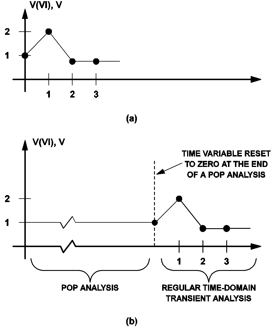 |
10.4 (a) Waveform of a sample piecewise-linear voltage source when no periodic operating point analysis is specified, and (b) Waveform of the same voltage source when a periodic operating point analysis is carried out. |
Periodic Sources
Periodic sources are left unchanged during a POP analysis, and the time variable is reset to 0.0 at the end of a POP analysis. However, it is not always true that the source value of a periodic source at the end of a POP analysis will be equal to the value of the same source at t = 0 as defined in the input file. The reason for this can be seen by examining the following statements in the input file:
VA 999 0 SAW V1=1 V2=3 FREQ=1K DELAY=0
+ OFF_UNTIL_DELAY=NO
VB 998 0 SAW V1=1 V2=3 FREQ=1K DELAY=250U
+ OFF_UNTIL_DELAY=NO
!DX 555 0 999 997 MX IC=0
.MODEL MX COMP RIN=10MEG ROUT=8 HYSTWD=2M
+ VOL=0 VOH=5
VDC 997 0 DC 1.999
.POP TRIG_GATE=!DX TRIG_COND=0_TO_1 MAX_PERIOD=400U
If no periodic operating point analysis is carried out, the source values V(VA) and V(VB) would be as shown in fig 10.5 (a). From this diagram, the source values V(VA) and V(VB) are obviously equal to 1V and 2.5 V, respectively, at t = 0. However, at the exit of a successful POP analysis, the source value of VA will be found to be equal to 2V rather than 1V. The cause of this discrepancy comes from the arbitrary reset of the time variable to zero at the end of the POP analysis. To understand this reasoning, the reader is referred to fig 10.5 (b), which shows the waveforms of V(VA), V(VB), and the logic output of the gate !DX. From the input file statements above and from fig 10.5 (b), the start of a switching cycle is seen to occur at time instants when V(VA) is rising and equal to 2V. Since each of the invisible transient analyses carried out in the periodic operating point analysis is terminated at the start of a new switching cycle, the source value V(VA) must be at 2V at the end of the POP analysis. Similarly, the source value V(VB) is equal to 1.5 V, rather than 2.5V, at the end of the POP analysis.
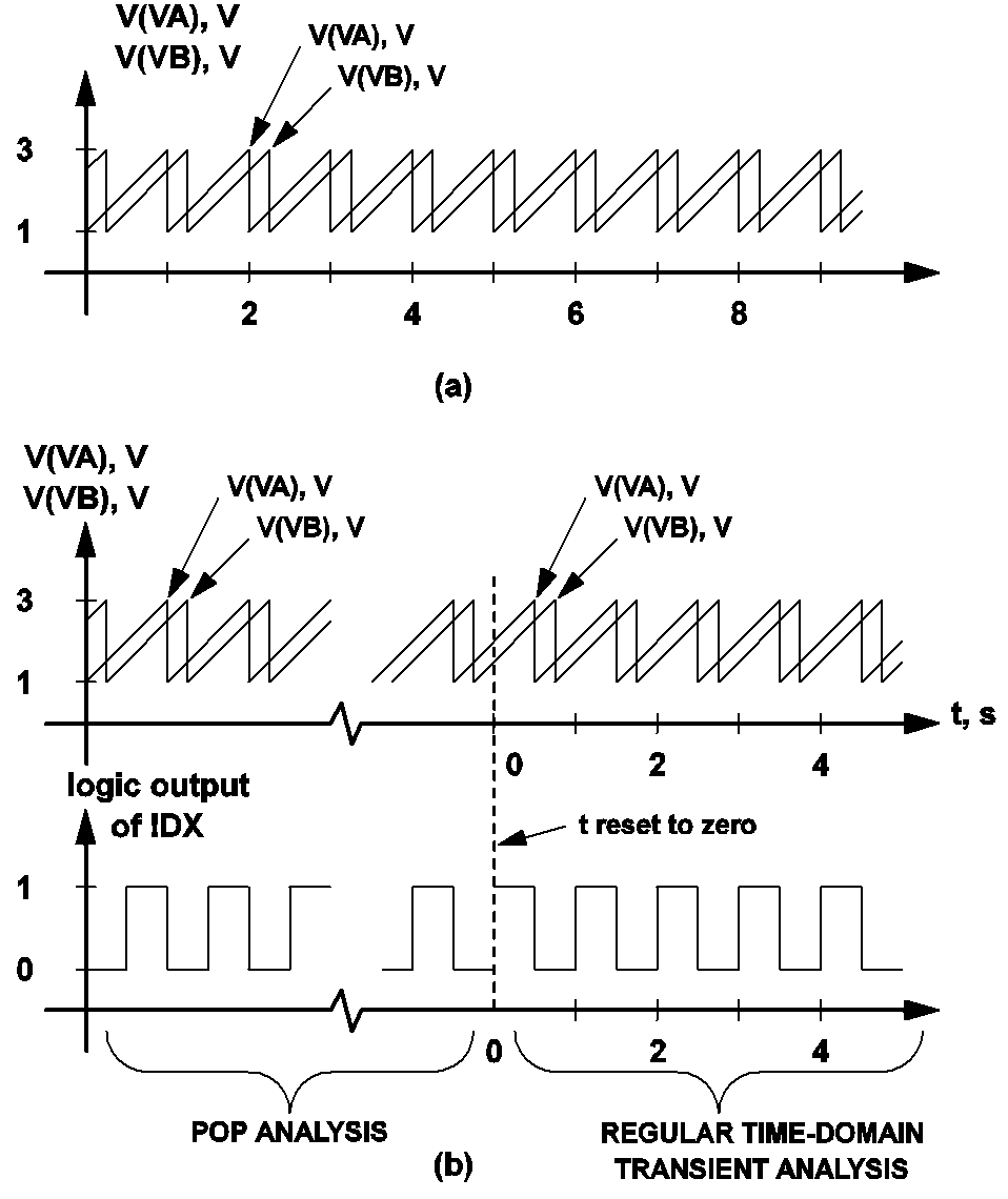 |
10.5 (a) Waveforms of two periodic sawtooth voltage sources VA and VB when no periodic operating point analysis is carried out, and (b) Waveform of the same voltage source when a periodic operating point analysis is carried out. The start of a switching cycle is defined as occurring when the output of the logic gate !DX is making a 0 to 1 transition. |
The POP_SHOWDATA option for POP Analysis
Under normal application of the periodic operating point analysis, the POP_SHOWDATA option should be turned off. If a POP analysis fails, the user can run a regular time-domain transient analysis, without the POP analysis, to make sure that the system has been correctly defined, modeled, and entered in the input file. Typographical errors in entering the initial conditions for some devices or mistakes in the definition of the switching logic can often be revealed through such a regular time-domain transient analysis.
After debugging the defined system to make sure initial conditions are within reasonable ranges and the switching logic is properly set up, the user can apply the POP analysis again to compute the steady-state solution. If the POP analysis fails again, the user may want to examine the progress of the POP analysis by repeating the POP analysis with the POP_SHOWDATA option turned on. When the POP_SHOWDATA option is turned on, a print/plot file named "XXXX.t4", where "XXXX" is the name of the input file, is generated during the POP analysis. This data file contains data for all of the print variables versus the time variable for the sequence of invisible transient analyses carried out by the POP analysis.
Due to the prediction phases interspersed between successive transient analyses, the time variable, as pointed out in See The Value of the Time Variable During the Periodic Operating Point Analysis , has no real physical meaning and significance because the POP analysis is not following any true transient experienced by the system. To make it easier to review the print variables in this data file, the time variable in this data file is artificially set so that 1) it appears to be continuous and monotonically increasing, and 2) the time instant at the end of each transient analysis carried out by the POP analysis also appears to be the instant at the start of the next transient analysis. Since the prediction phase carried out between two successive transient analyses adjusts the capacitor voltages and inductor currents so as to predict the steady-state solution, jump discontinuities in the print variables are expected in this data file at the boundary between successive switching cycles. As a result, it is not uncommon to see discontinuities in the capacitor voltages and inductor currents if a plot is made from this data file.
A typical waveform plotted from the "XXXX.t4" data file for a successful POP analysis is shown in fig 10.6 (a). The switching frequency for this example is 10 kHz and discontinuities in the waveform are observed at intervals of 100 microseconds. Typical waveforms plotted from the "XXXX.t4" data file for unsuccessful POP analyses are shown in fig 10.6 (b) and fig 10.6 (c). The waveform in fig 10.6 (b) is representative of a high-gain closed-loop regulated system where a small change in the capacitor voltages or inductor currents can cause a dramatic change in the mode of operation of the system. In such a case, the user may want to run a regular time-domain transient analysis until the system settles to a stable mode of operation, read off the capacitor voltages and inductor currents, and then run a POP analysis with the new initial conditions. The waveform in fig 10.6 (c) is representative of a system where the initial conditions for a few devices as supplied by the user in the input file are very far away from the values that they should be during steady-state operation. For instance, the waveform in fig 10.6 (c) suggests that, to approach steady-state operation, the initial condition associated with the capacitor CC should be increased to at least 100 V. Although the example waveforms shown in fig 10.6 are either capacitor voltages or inductor currents, all voltage and current variables specified in the .PRINT statement are generated in this data file for the user to examine the progress of the POP analysis.
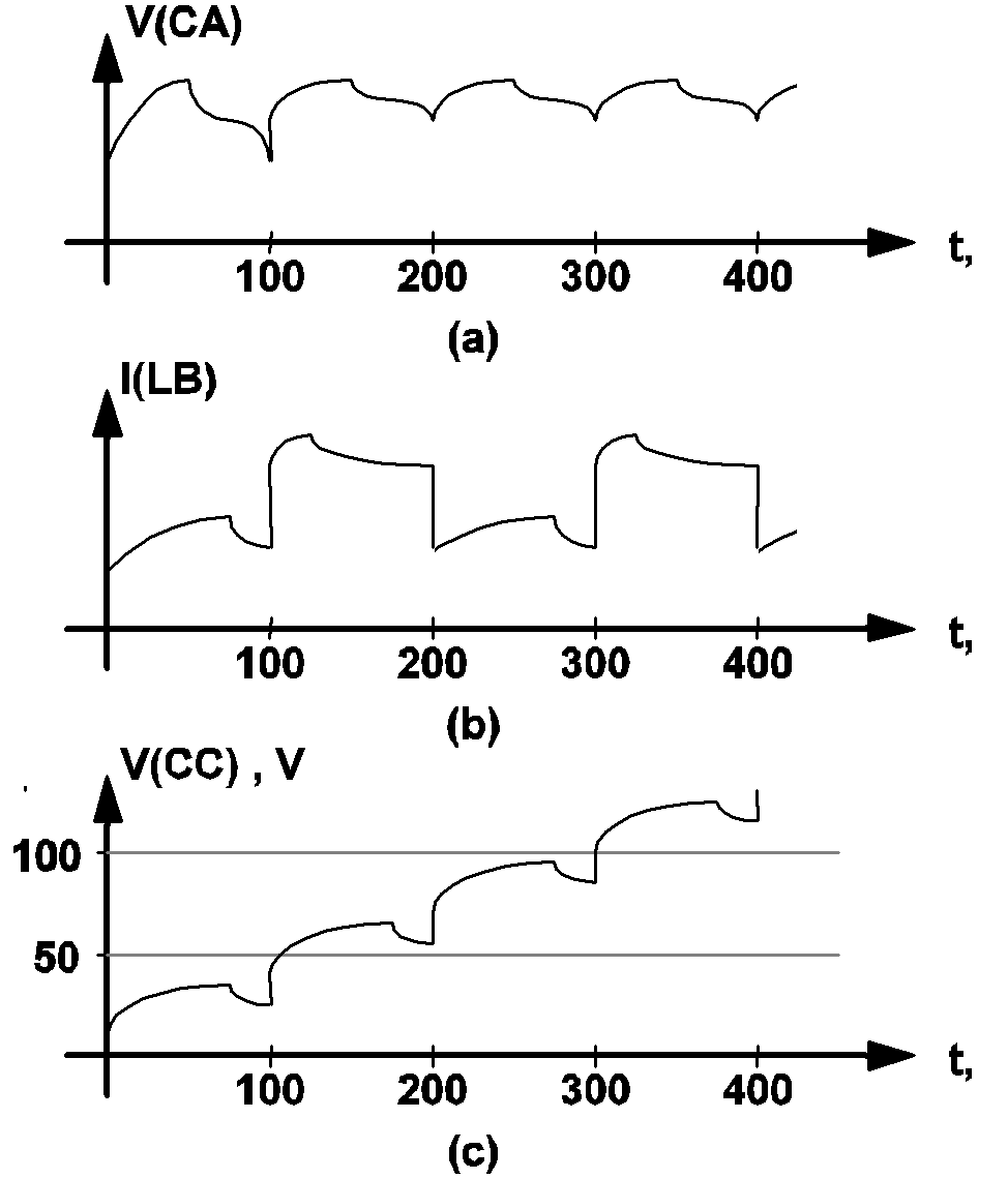 |
10.6 Typical waveforms obtained using the POP_SHOWDATA option:(a) Successful POP analysis, waveforms settle in a periodic steady state, (b) Unsuccessful POP analysis, waveforms fluctuate with large variations from one cycle to the next, and (c) Unsuccessful POP analysis, waveforms approach unilaterally, but do not settle in a periodic steady state. |
| ◄ Statements Relating to POP Analysis | Example of Applying the POP Analysis Tool ▶ |