1.0.2 PWL Simulation and Modeling
Every device model used in a SIMPLIS simulation uses Piecewise Linear (PWL) modeling techniques. This includes semiconductor devices such as MOSFETs and Diodes. In this topic you will learn how SIMPLIS models non-linear devices with PWL models.
In this topic:
Key Concepts
This topic addresses the following key concepts:
- Every model used in SIMPLIS is a Piecewise Linear (PWL) model.
- Non-linear characteristics are modeled with PWL primitive resistors, inductors or capacitors.
- Complex devices, such as MOSFETs can be represented by a collection of PWL devices.
- In SIMPLIS, diodes can be nothing more than PWL resistors.
What You Will Learn
In this topic, you will learn the following:
- How transformer saturation is modeled with PWL inductors.
- How SIMPLIS uses a collection of PWL devices to model a MOSFET.
Getting Started
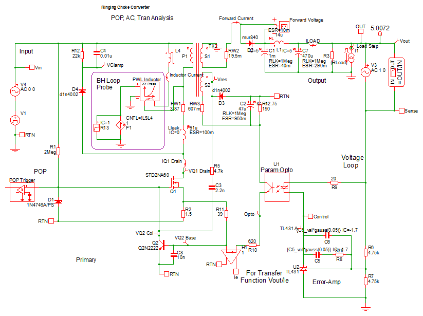
This topic uses a self-oscillating flyback converter to demonstrate PWL modeling techniques. The converter is intentionally overloaded, causing the converter to enter into a current limited operation. To get started with this example, follow these steps:
- Open the schematic titled
1.1_SelfOscillatingConverter_POP_AC_Tran.sxsch.Result: The flyback converter schematic opens:
- To simulate the design, press F9 or from the menu bar,
select .Result: After the simulation completes, the waveform viewer displays multiple graph tabs. If you have closed the waveform viewer or one of the graph tabs, run the simulation again to regenerate the graphs. The right-most two graphs are of interest, these two graph tabs will be similar to:
Time Domain Waveforms B-H Loop of Time Domain Model 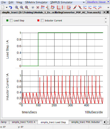
Discussion
PWL Inductors
The left hand graph contains two curves, the Load Step in green, and the Magnetizing Inductor Current in red.
During the transient simulation, a one amp load step is applied at 100us. During this load step, the total load current transitions from a 2A full load condition to a 3A overload condition with the consequence that the transformer enters into saturation. The current limit function is triggered and the output voltage drops.
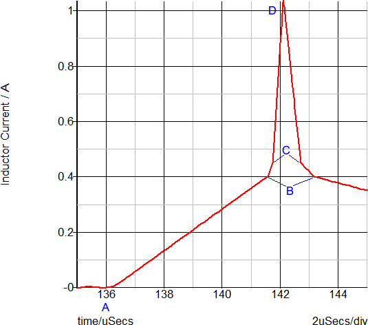
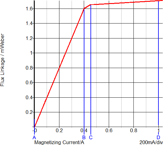
This overload condition demonstrates how a PWL inductor models transformer saturation. The following two graphs show a close-up view of the time-domain magnetizing inductor waveform and the flux linkage versus current plane on which PWL inductors are defined. Each of these three PWL inductor segments can be seen in both the transient simulation results and in the x-y plot of the flux linkage versus current plane show below:
| Saturating Magnetizing Current | B-H Loop |
|
|
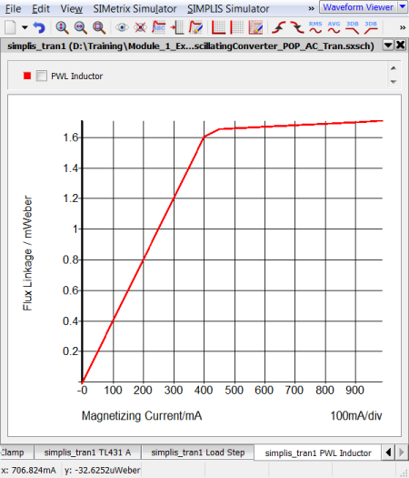
The saturation of this transformer is modeled with three PWL segments in the flux linkage versus current plane. Because the slope of this curve is the magnetizing inductance, the magnetizing inductance can take on three distinct values:
- When the magnetizing current is below 0.4A, the normal or unsaturated magnetizing inductance of 1.6mWeber/0.4A equals 4mH is used.
- The knee of saturation occurs when the magnetizing current is between 0.4 and 0.45A. The inductance in this region is (1.65m-1.6m)/(0.45-0.40) which equals 1mH.
- The final PWL segment represents a "hard" saturation. The inductance of this segment is 100uH.
PWL MOSFETs and Diodes
What about the Diodes and the MOSFET on the schematic? Are these PWL models as well? Yes!
- In SIMPLIS, the built-in diode models are nothing more than PWL resistors with either 2 or 3 segments. The PWL definition is usually generated with the automatic model parameter extraction routines built into SIMetrix/SIMPLIS.
- The built-in MOSFET models are made from a collection of PWL devices,
including:
- A PWL resistor representing the body diode
- A transistor switch with a constant forward transconductance gain (Gm)
- PWL capacitors representing the voltage dependent nonlinear capacitances.
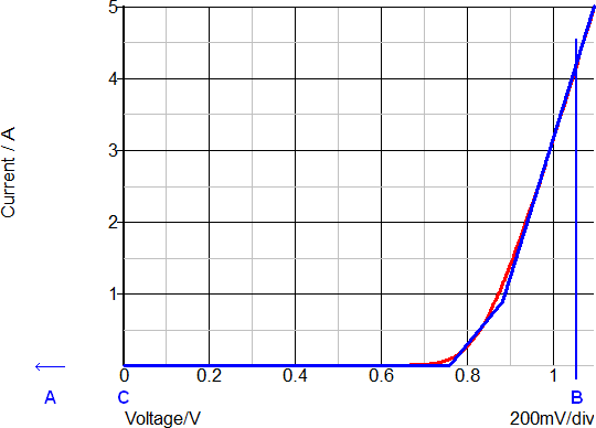
As an example, the output rectifier in the Self-Oscillating Converter has the following Forward Current and Forward Voltage curves during the transient simulation. The left hand graph has the Forward Current and Forward Voltage plotted vs. Time. In the right-hand graph, the Forward Current is plotted versus the Forward Voltage for this diode. The blue curve is the 3 segment SIMPLIS PWL model. The red curve is the SIMetrix simulation results for SPICE model of the same diode.
| Voltage and Current vs. Time | Voltage vs. Current |
|
|
|
The annotated points describe the following diode states:
- A: Blocking state
- B: Conducting 4A forward current
- C: Transition from conduction to blocking state
An in depth discussion of MOSFET modeling is presented in section 1.0.3 Multi-Level Modeling.
Conclusions and Key Points to Remember
- Every device used in a SIMPLIS simulation is, behind the scenes, a PWL model. This is independent of the symbol. The symbol is merely a graphical representation of the underlying function being modeled.
- The nonlinear characteristics of Resistors, Capacitors, and Inductors are modeled as a series of PWL straight line segments.
- Even complex devices, such as MOSFETs can be represented by a collection of PWL devices.