Continuous or Discrete Time Filter
The Continuous or Discrete Time Filter models either a continuous time filter or a discrete time filter, with a parameter editing dialog which calculates the coefficients. You can enter the coefficients for a s-domain or z-domain transfer function and the dialog will calculate an equivalent filter in the other domain using one of the three mapping functions.
These filters are available in 1st and 2nd order, as the models used for the discrete time filter are limited to the second order. Higher order filters can be realized by cascading two or more filters.
The electrical model used for these filters is either the Laplace Filters (1st, 2nd, 3rd Order) for a continuous time implementation, and for the discrete time implementation, the 1st Order Discrete Time Filter or 2nd Order Discrete Time Filter, depending on the filter order. The difference between this part and the Laplace and Discrete Time filters is the calculator dialog.
In this topic:
| Model Name: | Continuous or Discrete Time Filter | |||
| Simulator: | This device is compatible with the SIMPLIS simulator. | |||
| Parts Selector Menu Locations: |
|
|||
| Symbol Library: | simplis.sxslb | |||
| Model File: |
|
|||
| Subcircuit Names: | SIMPLIS_CONT_OR_DISCRETE_TIME_FILTER | |||
| Symbols: |
|
|||
| Multiple Selections: | Multiple devices can be selected and edited simultaneously. | |||
Converting a Continuous Time (s-domain) Transfer Function to the Z-Domain
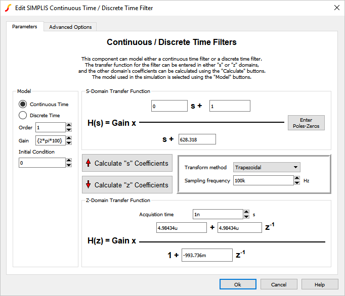
The filter has a calculator dialog which converts an s-domain transfer function to the z-domain or vice versa. This section assumes you have a s-domain transfer function which you would like to convert to the z-domain. To convert a z-domain transfer function to the s-domain, see Converting a Discrete Time (z-domain) Transfer Function to the S-Domain.
To configure the Continuous or Discrete Time Filter as a discrete-time filter, follow these steps:
- Double click the symbol on the schematic to open the editing dialog.
- On the editing dialog:
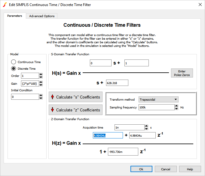
- Select the Discrete Time radio button.
- Select your desired filter order using the Order parameter.Result: The transfer functions to the right of the Order control are updated to reflect the current filter order.
- Enter the coefficients for your S-Domain Transfer Function for which you wish to calculate an equivalent z-domain transfer function. The coefficients can also be calculated by Entering Poles and Zeros for the S-Domain Transfer Function.
- Enter your Sampling frequency and select your desired Transform method.
- Click the Calculate "z" Coefficients button.Result: The Z Domain Transfer Function coefficients are updated with values calculated from the S-Domain Transfer Function coefficients.
- Click Ok.Result: The symbol on the schematic changes to a discrete time filter with input and output clock pins, and the equation is updated on the symbol. If multiple filters were selected, each filter symbol is replaced and each filter is identical.
Entering Poles and Zeros for the S-Domain Transfer Function
With the release of version 8.20, there exists an entry dialog, in which you can enter the Poles and Zeros of your S-Domain Transfer Function instead of the coefficients. The poles and zeros are entered in radians per second (ω); however, by setting the Frequency Scale Factor to 2*pi, the entries can be made in Hertz.
- Click the Enter Poles-Zeros button.
- On the editing dialog:
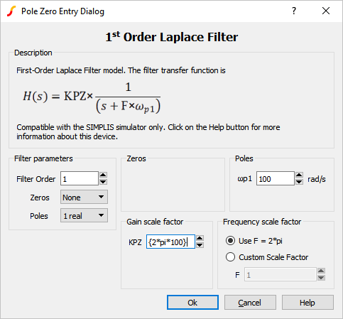
- Select the type and number of Zeros by using the Zeros drop down menu.
- Select the type and number of Poles by using the Poles drop down
menu.Result: The transfer function equation will update and the associated input boxes will appear.
- Enter the desired Poles and Zeros.
- Click Ok.Result: Focus will return to the Continuous/Discrete Time Filter dialog and the S-Domain Transfer Function coefficients will be calculated and populated.
Converting a Discrete Time (z-domain) Transfer Function to the S-Domain
The filter has a calculator dialog which converts an s-domain transfer function to the z-domain or vice versa. This section assumes you have a z-domain transfer function which you would like to convert to the s-domain. To convert a s-domain transfer function to the z-domain, see Converting a Continuous Time (s-domain) Transfer Function to the Z-Domain.
To configure the Continuous or Discrete Time Filter as a continuous-time filter, follow these steps:
- Double click the symbol on the schematic to open the editing dialog.
- On the editing dialog:
- Select the Continuous Time radio button.
- Select your desired filter order using the Order parameter.Result: The transfer functions to the right of the Order control are updated to reflect the current filter order.
- Enter the coefficients for your Z-Domain Transfer Function for which you wish to calculate an equivalent s-domain transfer function.
- Enter your Sampling frequency and select your desired Transform method.
- Click the Calculate "s" Coefficients button.Result: The S Domain Transfer Function coefficients are updated with values calculated from the Z-Domain Transfer Function coefficients.
- Click Ok.Result: The symbol on the schematic changes to a continuous time filter and the equation is updated on the symbol. If multiple filters were selected, each filter symbol is replaced and each filter is identical.
Parameter Editing Controls
The main parameter editing controls are described in the table below.
| Parameter Groupings/Labels | Units | Description |
| S-Domain Transfer Function | Enter the S-Domain filter coefficients in the text boxes. When you change the Order parameter, the equation and the available text boxes will change accordingly. Parameterized values using {} expressions are not permitted for these parameters. | |
| Enter Poles-Zeros | This button will open a dialog that will allow the entry of Poles and Zeros. The coefficients of the S-Domain Transfer Function will be calculated based on the desired Poles and Zeros. | |
| Z-Domain Transfer Function | Enter the Z-Domain filter coefficients in the text boxes. When you change the Order parameter, the equation and the available text boxes will change accordingly. Parameterized values using {} expressions are not permitted for these parameters. | |
| Calculate "s" Coefficients | This button uses the Z-Domain Transfer Function parameters, the Transform method, and the Sampling frequency to calculate an equivalent s-domain filter. | |
| Calculate "z" Coefficients | This button uses the S-Domain Transfer Function parameters, the Transform method, and the Sampling frequency to calculate an equivalent z-domain filter. | |
| Transform method | The transform method | |
| Sampling frequency | The sampling frequency for the discrete time filter. This is used to calculate both the s-domain and z-domain coefficients. Parameterized values using {} expressions are not permitted for this parameter | |
| Order | The filter order. Parameterized values using {} expressions are not permitted for this parameter | |
| Gain | The filter gain | |
| Initial Condition - IC | V | Initial output voltage of the filter |
The dialog has an Advanced Options tab with three controls which affect the precision of the model and the transfer function displayed on the symbol. There are text descriptions on the dialog tab to the right of each control which describe the control's function.
The pole-zero entry editing controls are described in the table below.
| Parameter Groupings/Labels | Units | Description |
| Description | The description of the filter including the transfer function in the Pole-Zero form. | |
| Order | The filter order. Parameterized values using {} expressions are not permitted for this parameter | |
| Filter Inputs - Zeros | Desired number of Zeros (real and complex) | |
| Filter Inputs - Poles | Desired number of Poles (real and complex) | |
| Zeros - ωz1 | rad/s | Desired zero location. Parameterized values using {} expressions are not permitted for this parameter |
| Zeros - ωz2 | rad/s | Desired zero location. Parameterized values using {} expressions are not permitted for this parameter |
| Zeros - ωzn | rad/s | Natural undamped frequency. Parameterized values using {} expressions are not permitted for this parameter |
| Zeros - ζz | Damping Ratio. Parameterized values using {} expressions are not permitted for this parameter | |
| Poles - ωp1 | rad/s | Desired pole location. Parameterized values using {} expressions are not permitted for this parameter |
| Poles - ωp2 | rad/s | Desired pole location. Parameterized values using {} expressions are not permitted for this parameter |
| Zeros - ωpn | rad/s | Natural undamped frequency. Parameterized values using {} expressions are not permitted for this parameter |
| Zeros - ζp | Damping Ratio. Parameterized values using {} expressions are not permitted for this parameter | |
| Gain Scale Factor - KPZ | Multiplier for gain | |
| Frequency Scale Factor - F | Multiplier for frequency. By setting this to 2*pi, the radian frequencies will be transformed into Hertz. Parameterized values using {} expressions are not permitted for this parameter |
Previous Version Compatibility
The subcircuit and editing dialog for the Continuous/Discrete Time filter were introduced in version 8.10. The filter will not simulate nor will it be editable in versions prior to 8.10.
For discrete time filters which are compatible with previous versions, see the part selector locations:
Examples
Below are two examples of varying complexity which demonstrate how to use the Continuous/Discrete Time filters.
Example - Simple 1st Order Filter with One Pole and One Zero
| simplis_081_continuous_time_pole_zero.sxsch | simplis_081_discrete_time_pole_zero.sxsch |
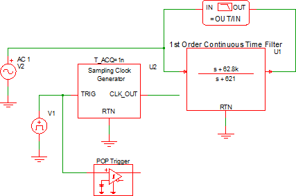 |
 |
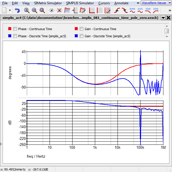
Waveforms - Simple 1st Order Filter with One Pole and One Zero
The schematics are configured to output the gain/phase waveforms to the same grid so the two filters can be easily compared. The AC response for the two filters is shown below:
Example - 1st Order Low Pass Filter (LPF)
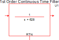
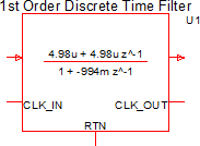
| simplis_081_continuous_time_lpf.sxsch | simplis_081_discrete_time_lpf.sxsch |
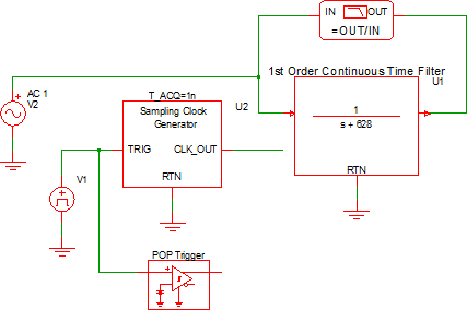 |
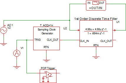 |
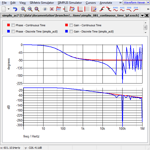
Waveforms - 1st Order Low Pass Filter (LPF)
The schematics are configured to output the gain/phase waveforms to the same grid so the two filters can be easily compared. The AC response for the two low pass filters is shown below: