Application E - Digital Control: Convert Analog Compensation Network to Digital Compensation Network
SIMetrix/SIMPLIS provides users the ability to model their digital components in a variety of ways. The four ways of modeling a digital component are by using digital hardware, discrete-time filters, SystemDesigner devices, and Verilog-HDL. This topic describes how to convert an existing analog compensator to a digital PID compensator using both discrete-time filters and SystemDesigner devices.
To download the examples for the Applications Module, click Applications_Examples.zip.
In this topic:
Key Concepts
This topic addresses the following key concepts:
- Converting an existing Type III analog compensation network to a digital compensation network using both discrete time filters and SystemDesigner components.
What You Will Learn
Using a step-by-step procedure, you will convet an anolog Type III compensator to a digital PID compensator.
In this topic, you will learn the following:
- Two methods for calculating 2nd Order Discrete Filter coefficients
- How to use the Continuous or Discrete Time Filter model
- Multiple ways to impliment a digital circuit design.
Design Procedure
The design procedure for this application uses the following steps.
- Step 1a: Determine the S-Domain equivalent of your analog compensation network
- Step 1b: Replace the existing compensation network with the new S-Domain equivalent
- Step 2: Determine discrete time component coefficients
- Step 3: Replace S-Domain equivalent network with high-level discrete time components
- Step 4: Build up digital compensation network with discrete time building blocks to check accuracy
- Step 5a: Replace discrete time components with SystemDesigner components
- Step 5b: Prepare SystemDesigner circuit for Signed Integer simulation
Step 1a: Determine the S-Domain equivalent of your analog compensation network
We will begin with a Type III analog compensator:
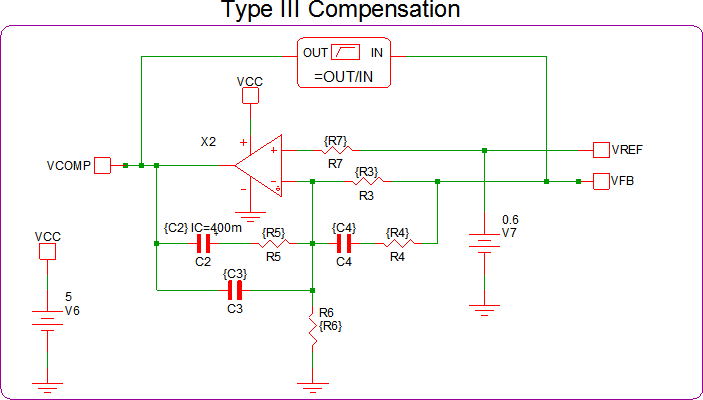
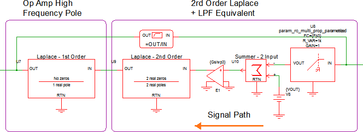
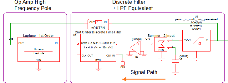
The Type III analog compensator has 3 poles and 2 zeros, therefore, a 3rd order laplace filter is needed. However, digital compensation networks require an anti-aliasing filter to be placed at its input. Therefore, we will remove one of the poles from the 3rd order laplace filter to use as an anti-aliasing filter. Thus resulting in a 2nd order laplace filter in series with a 1st order low-pass filter. Since the OpAmp in this example is not ideal, an additional 1st order laplace filter with 1 real pole at 700kHz and no zeros is used to model the high frequency behavior of the OpAmp. The equivalent filter schematic is shown below:
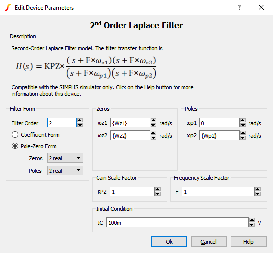
The second order laplace is set up as follows:
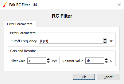
The anti-aliasing filter is set up as follows:
Below are all of the calculations for all of the variables:
\[ Gs = \frac{R_3+R_4}{R_3*R_4*C_3} \]
\[ \omega_{z1} = \frac{1}{(R_3+R_4)*C_4} \text{ , } \omega_{z2} = \frac{1}{R_5*C_2} \]
\[ \omega_{p1} = 0 \text{ , } \omega_{p2} = \frac{C_2+C_3}{R_5*C_2*C_3} \text{ , } \omega_{p3} = \frac{1}{R_4*C_4} \]
\[ f_{zn} = \frac{\omega_{zn}}{2*\pi} \text{ , } f_{pn} = \frac{\omega_{pn}}{2*\pi} \]
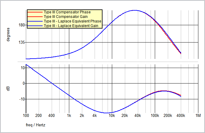
The AC results of the existing Type III compensation and the new 2nd Order Laplace equivalent are compared here:
Step 1b: Replace the existing compensation network with the new S-Domain equivalent
Now that you have an equivalent laplace based compensation network, you can replace your existing Type III compensator. The Type III - Laplace Filter equivalent circuit will remain in the circuit for later comparison.
Pole Location Talking Point
At this point, it would be good to talk about how the location of your poles in the frequency domain affect the steps going forward. If any of your poles are a greater frequency than ???MATH???fsw/\pi???MATH???, when the bilinear transformation occurs, said pole will be mapped to the Left Hand Plane (LHP) of the Z-Domain. When there is a pole in the Z-Domain LHP, the circuit will begin to oscillate and/or become unstable, even if your circuit is stable in the S-Domain.
If your calculated high frequency pole is greater than ???MATH???fsw/\pi???MATH???, it is recommended to lower that pole frequency. If that is not possible, or not desirable, when you perform the bilinear transformation and calculate your PID values, set the gamma (???MATH???\gamma???MATH???) value so that it satisfies the minimum requirements noted by equation 8 in the PID Discrete Time Filter documentation.
Step 2: Determine discrete time component coefficients
Determining your PID coefficients can be completed using one of two methods:
- Use the new (v8.10) Continuous or Discrete Time Filter model.
- Use a 3rd party software (GNU Octave, et al.)
Determining your PID coefficients - Method 1:
Method 1 involves using the new Continuous or Discrete Time Filter model released in version 8.10. The Continuous or Discrete Time Filter models either a continuous time filter or a discrete time filter, with a parameter editing dialog which calculates the coefficients. You can enter the coefficients for a s-domain or z-domain transfer function and the dialog will calculate an equivalent filter in the other domain.
In the F11 window of apps_e_step_1b_replace_type_iii_w_laplace.sxsch, you will see there are some statements that will allow you to calculate the numerator and denominator coefficients of the 2nd order laplace filter. The image below, from the F11 window of apps_e_step_2_discrete_time_filter.sxsch, shows these statements and the calculated results:
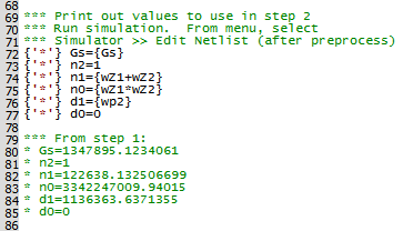
Using these calculations, copy and paste the numerator and denominator coefficients into the Continuous or Discrete Time Filter model dialog as shown below. The sampling frequency and acquistion time need to be also set before the "z" coefficients are calculated.
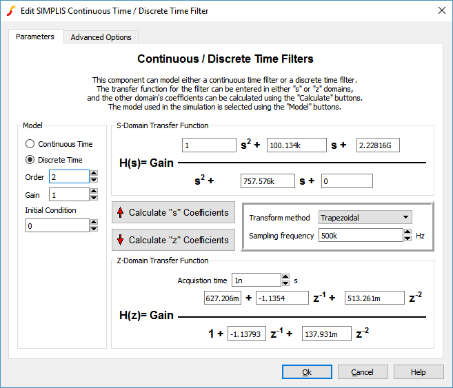
The Continuous or Discrete Time Filter model symbol will show the calculated discrete time equation:
From this point, you now need to calculate the roots of the numerator. Once you find the roots (???MATH???Z_1???MATH??? and ???MATH???Z_2???MATH???) the PID coefficients can be calculated as follows:
- ???MATH???K_d = Z_1*Z_2???MATH???
- ???MATH???K_p = Z_1+Z_2-2*Z_1*Z_2???MATH???
- ???MATH???K_i = 1+Z_1*Z_2-Z_1-Z_2???MATH???
From the ???MATH???H(z)???MATH??? equation above, you will need to extract two pieces of information. The first coefficient of the ???MATH???H(z)???MATH??? equation above will be multiplied into the existing LPF gain and the last denominator coefficient will be set as the Pole Factor (???MATH???\gamma???MATH???) of the PID filter.
Determining your PID coefficients - Method 2:
Method 2 involves using third party software. Any software that has the capabilities of calculating a bilinear transform and the roots of a second order polynomial will work. The software used for this application was GNU Octave. The calculations needed are identical to Method 1, however, they can all be completed at once. The calculations used in the example circuits can be downloaded here.
The AC results of the Type III Laplace Filter equivalent (from Step 1) and the new discrete time filter compensation are compared here:
Step 3: Replace S-Domain equivalent network with high-level discrete time components
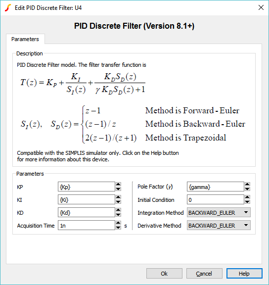
Now that you have the necessary coefficients, you can test them out using a PID Discrete Time Filter. Just as before, a PID fitler has been placed in apps_e_step_3_discrete_pid_filter.sxsch to test the PID coefficients.
The PID coefficients are placed in the F11 window and the PID dialog is set up as follows:
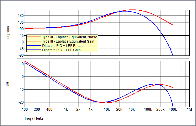
The AC results of the Type III Laplace Filter equivalent (from Step 1) and the new PID Filter compensation are compared here:
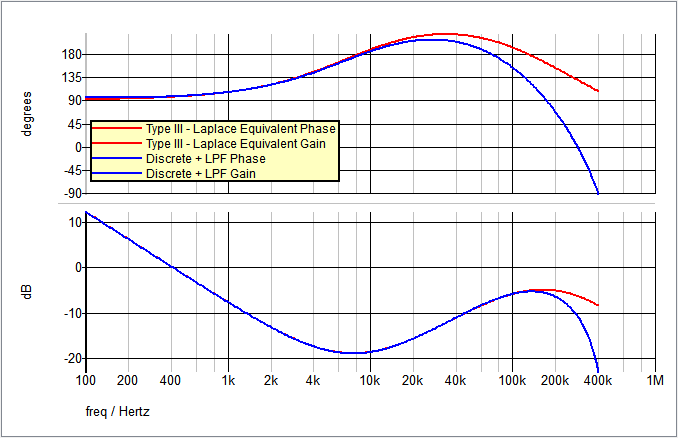
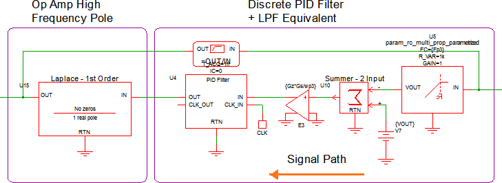
Step 4: Build up digital compensation network with discrete time building blocks to check accuracy
After confirming the accuracy of the calculated PID coefficients, the next
step is to break apart the discrete PID Filter into disrete time building blocks. For this
step, the Backward-Euler transform method will be used. The block diagram for this
transfrom method is as follows: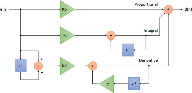
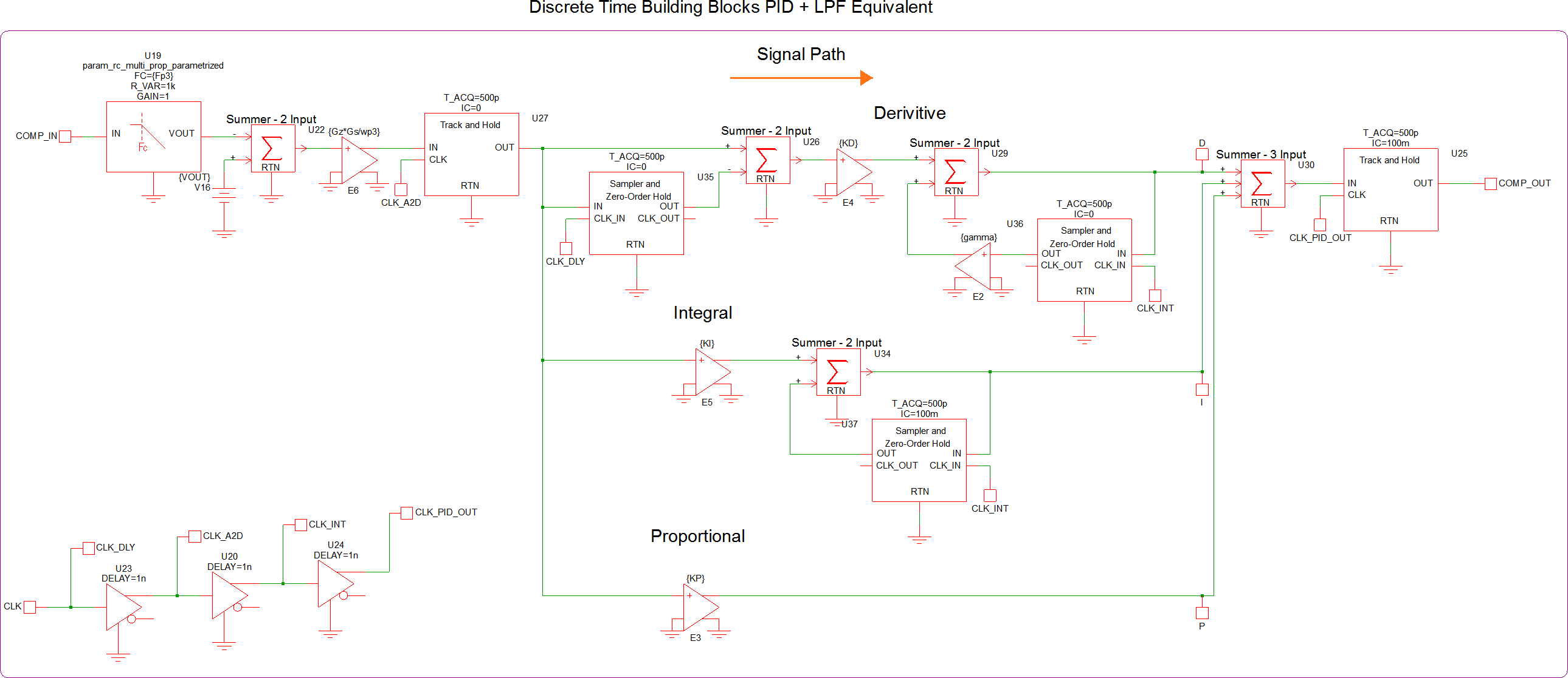
In apps_e_step_4_discrete_pid_filter_blocks.sxsch, each of the blocks in the diagram above are easily replaced with discrete time blocks:
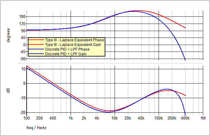
The AC results of the Type III Laplace Filter equivalent (from Step 1) and the new PID Filter compensation are compared here:
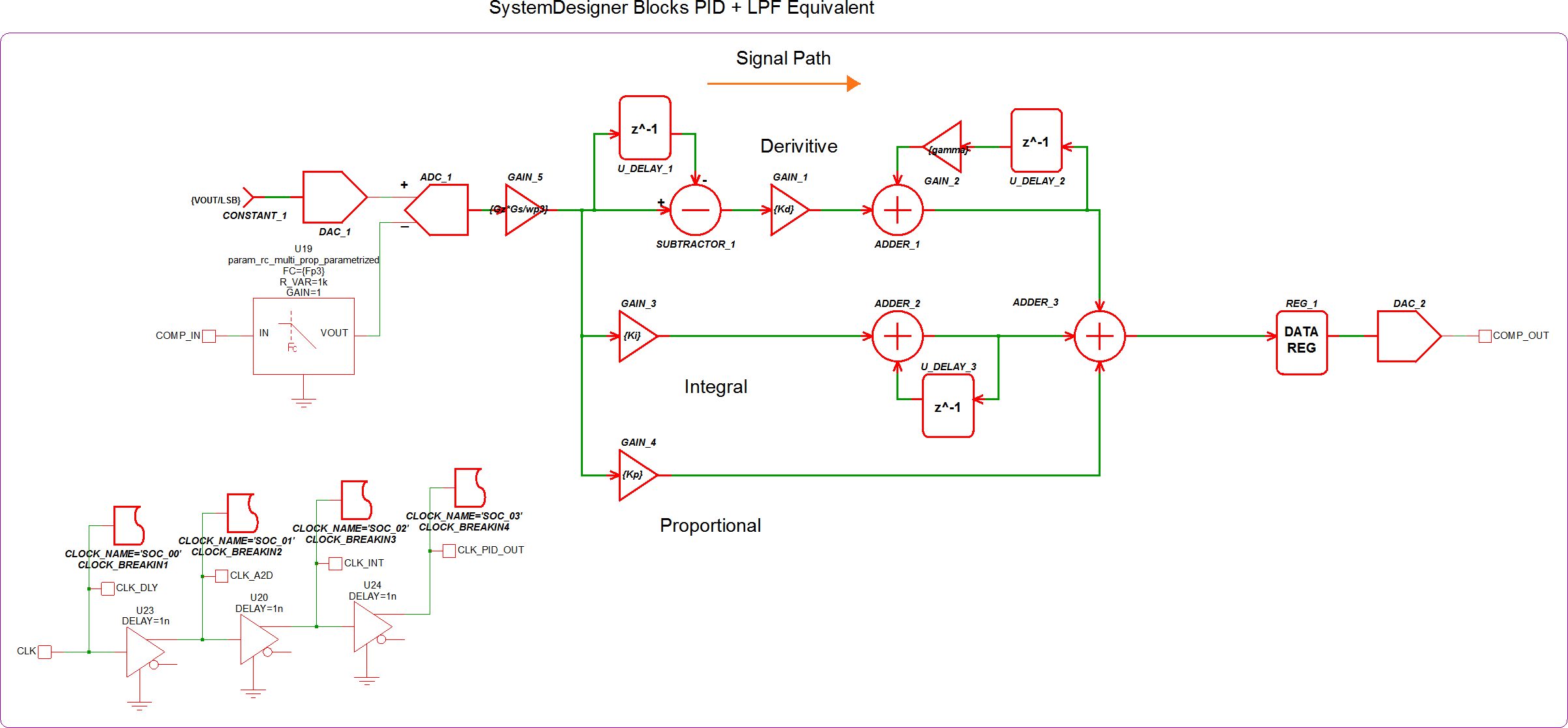
Step 5a: Replace discrete time components with SystemDesigner components
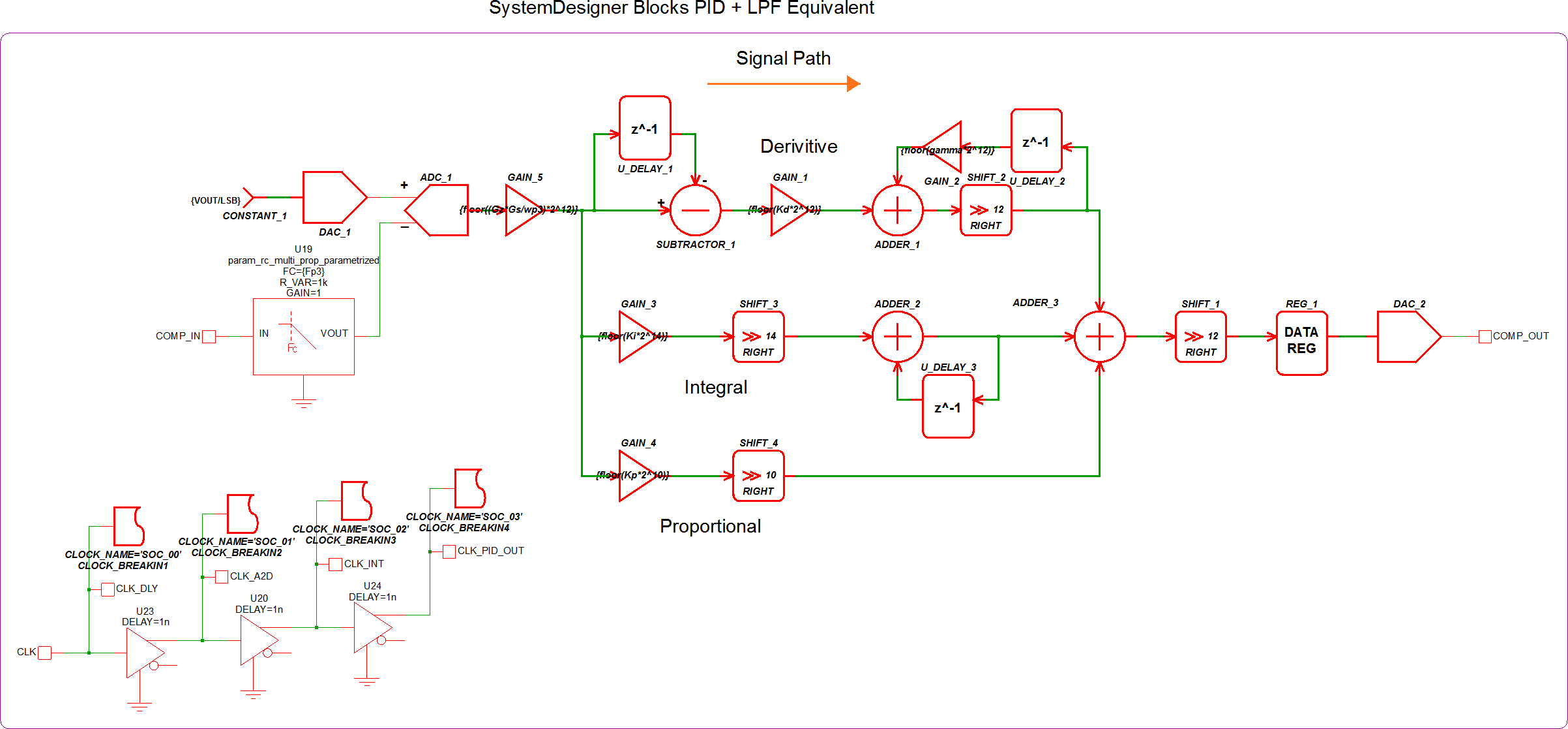
The first objective in step 5 is to switch out all of the discrete time components with their SystemDesigner equivalents and prepare the circuit to simulate with Double Precision Floating Point math. This simulation will allow you to run an AC analysis and check the accuracy of your circuit. The circuit in apps_e_step_5a_sd_pid_filter.sxsch is set up to run an AC analysis with the following SystemDesigner PID implimentation:
The AC results of the Type III Laplace Filter equivalent (from Step 1) and the new SystemDesigner PID Filter compensation are compared here:
Step 5b: Prepare SystemDesigner circuit for Signed Integer simulation
The final step in the process can be quite difficult and my require some trial-and-error. In order to run a Signed Integer simulation, the SystemDesigner blocks all must use only Integers. This can be done by multiplying the values that are less than 0 by a large number (more detail on this next) and then using the floor() function to round down to an integer value. The full PID circuit can be seen in the circuit apps_e_step_5b_sd_pid_filter_with_shifts.sxsch.
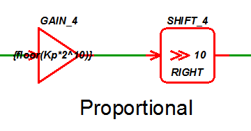
For more detail, we will examine the Proportial leg of the PID compensator. The calculated ???MATH???K_p???MATH??? value in this example is 0.173585978182213. From here, we have to determine how "large" of a number we need to mutiply ???MATH???K_p???MATH??? by in order to lessen the amount of error that is introduced when converting to an integer. You also want to multiply by a number that is equal to ???MATH???2^n???MATH??? so that you can use the Right Shift SystemDesigner component. A Right Shift is the same as dividing by ???MATH???2^n???MATH???, where ???MATH???n???MATH??? is the number of bits. In this example, we chose ???MATH???n=10???MATH???:
After multiplying by ???MATH???2^{10}???MATH??? and applying the floor() function, the new value of the gain block is 177.
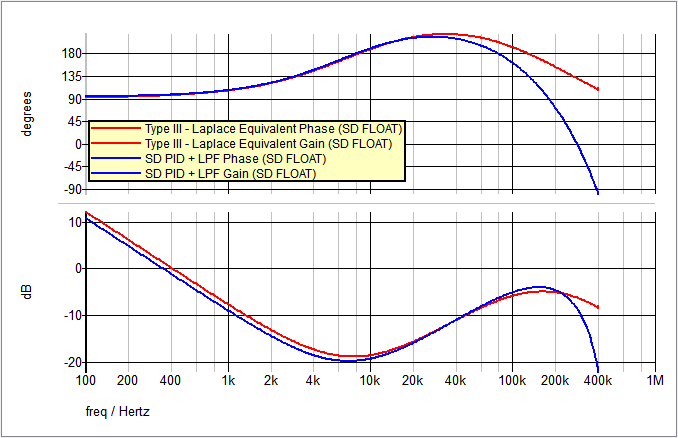
The AC results of the Type III Laplace Filter equivalent (from Step 1) and the new SystemDesigner PID Filter compensation are compared here:
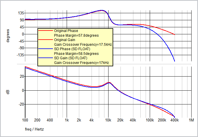
The closed loop AC results of the original circuit with the analog compensation network and the new PID Filter compensation are compared here:
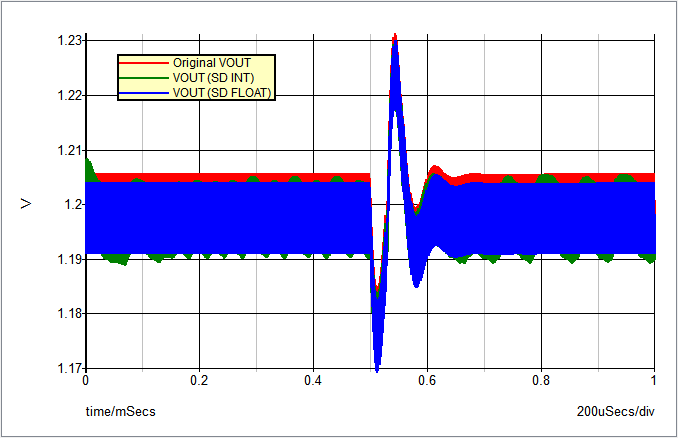
A final comparison is the Transient simulation. In the image below, you can see the red waveform is the original output voltage, the green waveform is the SystemDesigner Signed Integer mode output voltage, and the blue waveform is the SystemDesigner Double Precision Floating Point mode output voltage.
Conclusions and Key Points to Remember
- There are multiple ways to impliment a digital circuit design.
- The Continuous or Discrete Time Filter model can be used to convert an S-Domain transfer function to a Z-Domain transfer function.